inlabru interface

Introduction

The excursions package can also be used to analyze results obtained using inlabru. An advantage with inlabru is that it usually simplifies the model specification compared with plain INLA. To analyze inlabru outputs, the functions excursions.inla, simconf.inla and contourmap.inla can be used. Let us illustrate this using simulated data.

Let us generate some data

n.lattice <- 30
x <- seq(from = 0, to = 10, length.out = n.lattice)
lattice <- fm_lattice_2d(x = x, y = x)
mesh <- fm_rcdt_2d_inla(lattice = lattice, extend = FALSE, refine = FALSE)

sigma2.e <- 0.1
n.obs <- 100
obs.loc <- cbind(
  runif(n.obs) * diff(range(x)) + min(x),
  runif(n.obs) * diff(range(x)) + min(x)
)
Q <- fm_matern_precision(mesh, alpha = 2, rho = 3, sigma = 1)
x <- fm_sample(n = 1, Q = Q)
A <- fm_basis(mesh, loc = obs.loc)
Y <- as.vector(A %*% x + rnorm(n.obs) * sqrt(sigma2.e))

We now fit the model using rSPDE and inlabru. If we want to obtain an excursion set of the linear predictor evaluated at the mesh, the simplest option is to define a likelihood component in the bru call which contains NA observations at the mesh locations. We then give this component a tag (pred below) so that we can access these later.

rspde_model <- rspde.matern(mesh = mesh, nu = 1.5)
data <- data.frame(x1 = obs.loc[, 1], x2 = obs.loc[, 2], y = Y)
coordinates(data) <- c("x1", "x2")

# data for prediction locations
data.prd <- data.frame(
  x1 = mesh$loc[, 1],
  x2 = mesh$loc[, 2],
  y = rep(NA, dim(mesh$loc)[1])
)
coordinates(data.prd) <- c("x1", "x2")

cmp <- y ~ Intercept(1) + field(coordinates, model = rspde_model)
result_bru <- bru(~ Intercept(1) + field(coordinates, model = rspde_model),
  like(y ~ ., family = "normal", data = data),
  like(y ~ ., family = "normal", data = data.prd, tag = "prd"),
  options = list(
    control.compute = list(return.marginals.predictor = TRUE),
    num.threads = "1:1"
  )
)
#> Warning: `like()` was deprecated in inlabru 2.12.0.
#> ℹ Please use `bru_obs()` instead.
#> This warning is displayed once per session.
#> Call `lifecycle::last_lifecycle_warnings()` to see where this warning was
#> generated.
#> Warning: The `data` argument of `bru_obs()` has deprecated support for `Spatial` input
#> as of inlabru 2.12.0.9023.
#> ℹ Please use `sf` input instead.
#> ℹ The deprecated feature was likely used in the base package.
#>   Please report the issue to the authors.
#> This warning is displayed once per session.
#> Call `lifecycle::last_lifecycle_warnings()` to see where this warning was
#> generated.
#> Warning: Using `as.character()` on a quosure is deprecated as of rlang 0.3.0. Please use
#> `as_label()` or `as_name()` instead.
#> This warning is displayed once every 8 hours.

We can now compute excursion sets using the excursions.inla function. As no stack object is constructed when using inlabru, we use the argument name = "APredictor" to tell the function that we are interested in the linear predictor. We then use the bru_index function to obtain the indices for the relevant part of the predictor. In this case, we want the indices which correspond to the likelihood component which we gave the tag "pred" above, so the call looks as follows.

res.qc_bru <- excursions.inla(result_bru,
  name = "APredictor",
  ind = bru_index(result_bru, "prd"),
  alpha = 0.99, u = 0,
  method = "QC", type = ">",
  prune.ind = TRUE,
  max.threads = 2
)

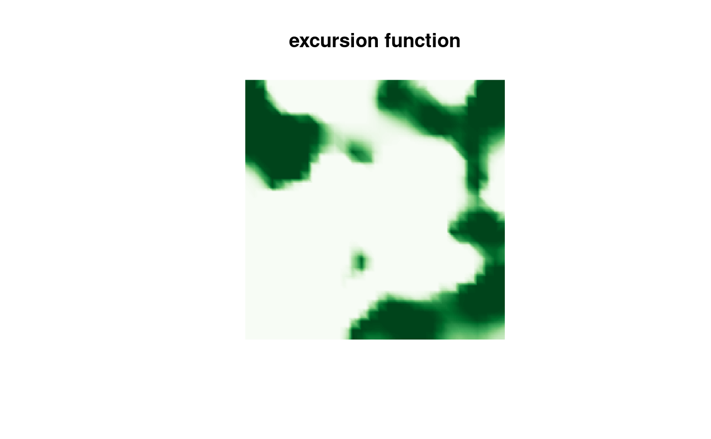
Note that we here set prune.ind = TRUE which tells the function that we want the result object only evaluated at the indices specified by the ind argument. We can now obtain a continuous domain representation through the continuous function

sets <- continuous(res.qc_bru, mesh, alpha = 0.1)

Finally, we can plot the results

cmap.F <- colorRampPalette(brewer.pal(9, "Greens"))(100)
proj <- fm_evaluator(sets$F.geometry, dims = c(300, 200))
image(proj$x, proj$y, fm_evaluate(proj, field = sets$F),
  col = cmap.F, axes = FALSE, xlab = "", ylab = "", asp = 1,
  main = "excursion function"
)

comparison of the different types of approximations

Above we used the QC method to compute the set. Let us now try the other available options and compare their timings and results.

t.EB <- system.time({
  res.EB <- excursions.inla(result_bru,
    name = "APredictor",
    ind = bru_index(result_bru, "prd"),
    alpha = 0.99, u = 0,
    method = "EB", type = ">",
    prune.ind = TRUE,
    max.threads = 2
  )
})
t.QC <- system.time({
  res.QC <- excursions.inla(result_bru,
    name = "APredictor",
    ind = bru_index(result_bru, "prd"),
    alpha = 0.99, u = 0,
    method = "QC", type = ">",
    prune.ind = TRUE,
    max.threads = 2
  )
})
t.NI <- system.time({
  res.NI <- excursions.inla(result_bru,
    name = "APredictor",
    ind = bru_index(result_bru, "prd"),
    alpha = 0.99, u = 0,
    method = "NI", type = ">",
    prune.ind = TRUE,
    max.threads = 2
  )
})
t.NIQC <- system.time({
  res.NIQC <- excursions.inla(result_bru,
    name = "APredictor",
    ind = bru_index(result_bru, "prd"),
    alpha = 0.99, u = 0,
    method = "NIQC", type = ">",
    prune.ind = TRUE,
    max.threads = 2
  )
})

The computation time for the different methods are

print(data.frame(
  time = c(t.EB[3], t.QC[3], t.NI[3], t.NIQC[3]),
  row.names = c("EB", "QC", "NI", "NIQC")
))
#>        time
#> EB    0.320
#> QC    0.538
#> NI   11.691
#> NIQC 10.344

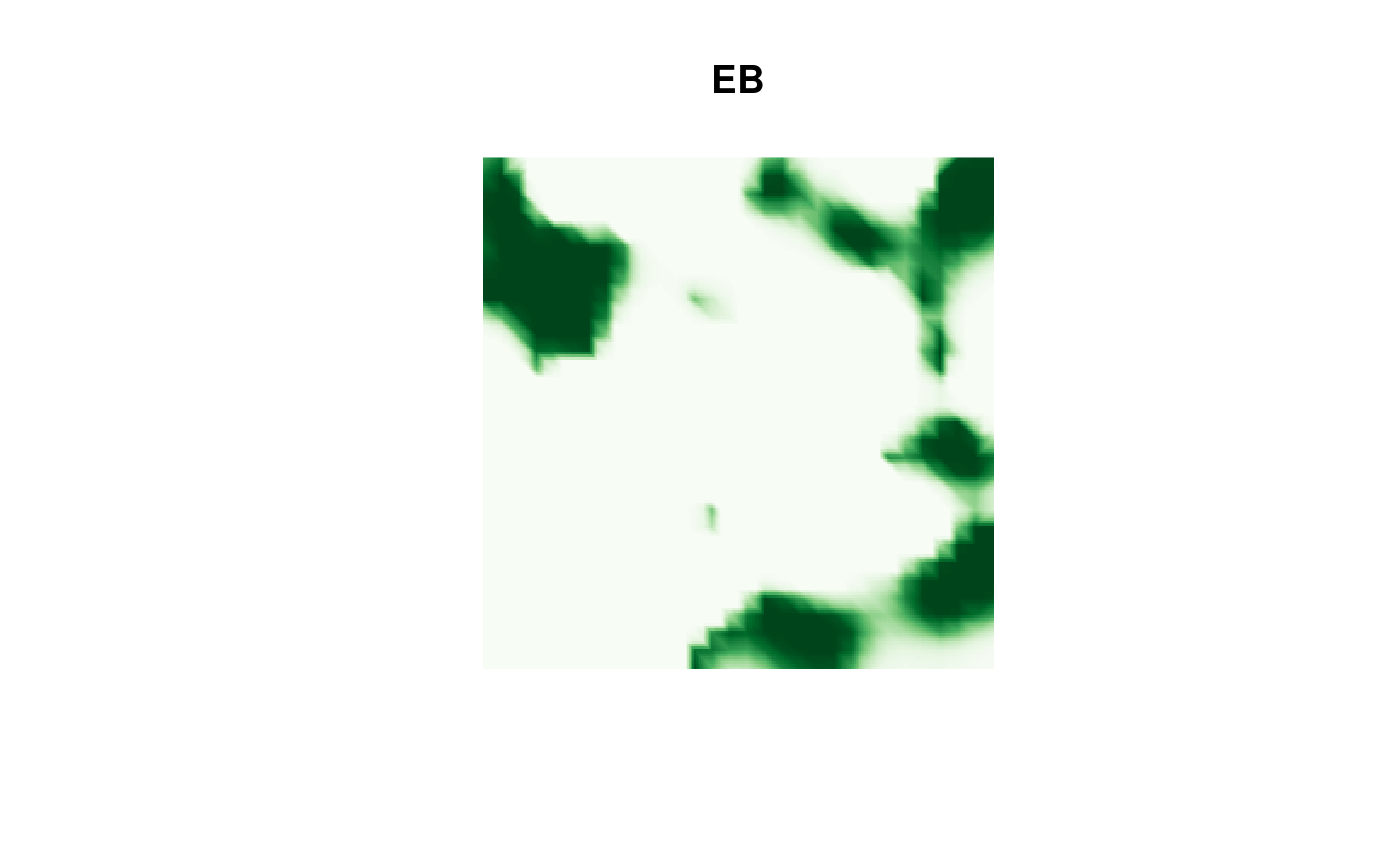
We can see that the EB and QC methods have similar computation times and that NI and NIQC take longer. Let us now plot the corresponding sets, we start with the EB result:

image(proj$x, proj$y, fm_evaluate(proj,
  field = continuous(res.EB,
    mesh,
    alpha = 0.1
  )$F
),
col = cmap.F, axes = FALSE, xlab = "", ylab = "", asp = 1,
main = "EB"
)

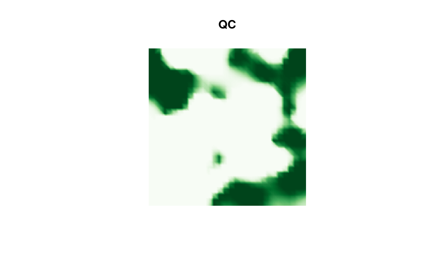
Then the QC result:

image(proj$x, proj$y, fm_evaluate(proj,
  field = continuous(res.QC,
    mesh,
    alpha = 0.1
  )$F
),
col = cmap.F, axes = FALSE, xlab = "", ylab = "", asp = 1,
main = "QC"
)

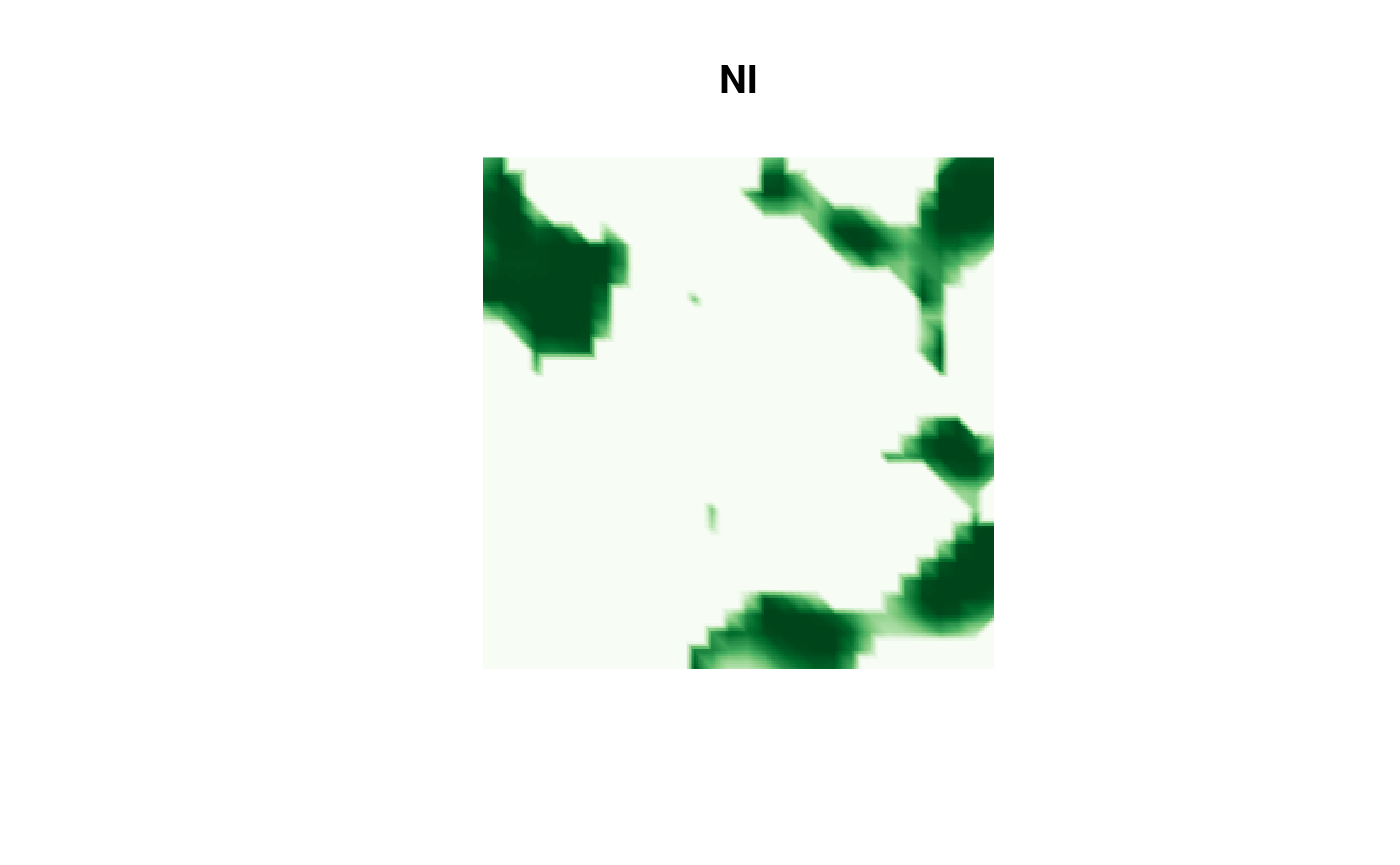
Then the NI result:

image(proj$x, proj$y, fm_evaluate(proj,
  field = continuous(res.NI,
    mesh,
    alpha = 0.1
  )$F
),
col = cmap.F, axes = FALSE, xlab = "", ylab = "", asp = 1,
main = "NI"
)

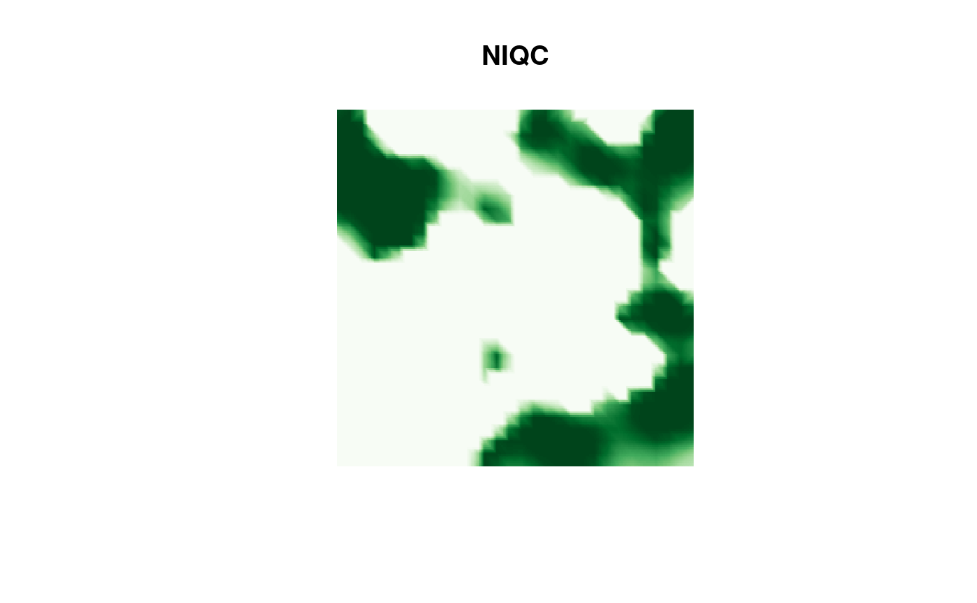
and finally the NIQC result:

image(proj$x, proj$y, fm_evaluate(proj,
  field = continuous(res.NIQC,
    mesh,
    alpha = 0.1
  )$F
),
col = cmap.F, axes = FALSE, xlab = "", ylab = "", asp = 1,
main = "NIQC"
)

Connected excursion regions

The excursion set is not necessarily connected. To instead compute connected regions where the field, with probability at least $1-\alpha$ , exceeds the level, we can use excursions.regions.inla, which is the INLA version of excursions.regions, see the getting started vignette for details. The function first computes the largest connected region, then removes its nodes and computes the largest region in the remaining nodes, and so on, which gives a map of non-overlapping connected regions that each satisfy the probability requirement.

The model is specified in the same way as for excursions.inla. In addition, the graph argument specifies which nodes are neighbours. Since the "prd" likelihood component contains one observation for each node of the mesh, in the same order, we can use the mesh as the graph. We only compute regions with at least 10 nodes.

reg_bru <- excursions.regions.inla(result_bru,
  name = "APredictor",
  ind = bru_index(result_bru, "prd"),
  graph = mesh,
  alpha = 0.1, u = 0,
  method = "QC", type = ">",
  min.size = 10,
  prune.ind = TRUE,
  max.threads = 2,
  seed = 1
)
lengths(reg_bru$regions)
#> [1] 64 41 33 31 19 12
reg_bru$P
#> [1] 0.9002252 0.9031823 0.9023169 0.9081605 0.9106351 0.9062027

As we used prune.ind = TRUE, the regions are given as indices of the mesh nodes. We compute continuous domain versions of the regions using continuous, and plot their outlines on top of the excursion function that we computed above, where each region has its own colour.

sets.reg <- continuous(reg_bru, mesh)
reg.col <- brewer.pal(8, "Set1")
image(proj$x, proj$y, fm_evaluate(proj, field = sets$F),
  col = cmap.F, axes = FALSE, xlab = "", ylab = "", asp = 1,
  main = "Connected regions"
)
plot(sets.reg$M,
  border = reg.col[(as.numeric(names(sets.reg$M)) - 1) %% 8 + 1],
  lwd = 2, add = TRUE
)

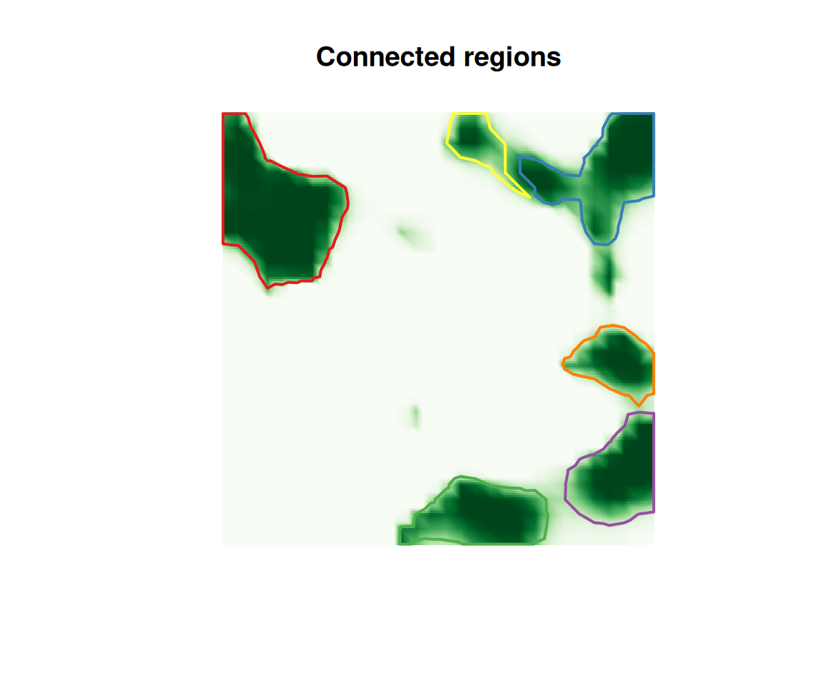Each region individually has a joint probability of at least $0.9$ of exceeding the level, whereas the excursion set, and thereby the excursion function, is defined through the joint probability for the whole set. A region can therefore contain nodes where the excursion function is below $0.9$ . For the same reason, two regions can be adjacent: their union is connected, but it does not satisfy the probability requirement jointly.

David Bolin and Finn Lindgren

Introduction

comparison of the different types of approximations

Connected excursion regions