Calculating probabilistic excursion sets and related quantities using excursions

David Bolin and Finn Lindgren

The functions in excursions can be divided into four main categories depending on what they compute: (1) Excursion sets and credible regions for contour curves, (2) Quality measures for contour maps, (3) Simultaneous confidence bands, and (4) Utility such as Gaussian integrals and continuous domain mappings. The main functions come in at least three different versions taking different input: (1) The parameters of a Gaussian process, (2) results from an analysis using the INLA software package, and (3) Monte Carlo simulations of the process. These different categories are described in further detail below.

As an example that will be used to illustrate the methods in later sections, we generate data $Y_i \sim N(X({\boldsymbol{\mathrm{s}}}_i),\sigma^2)$ at some locations ${\boldsymbol{\mathrm{s}}}_1, \ldots, {\boldsymbol{\mathrm{s}}}_{100}$ where $X({\boldsymbol{\mathrm{s}}})$ is a Gaussian random field specified using a stationary SPDE model (Finn Lindgren, Rue, and Lindström 2011).

x <- seq(from = 0, to = 10, length.out = 20)
mesh <- fm_rcdt_2d_inla(lattice = fm_lattice_2d(x = x, y = x),
                        extend = FALSE, refine = FALSE)
Q <- fm_matern_precision(mesh, alpha = 2, rho = 3, sigma = 1)
x <- fm_sample(n = 1, Q = Q)
obs.loc <- 10 * cbind(runif(100), runif(100))

Based on the observations, we calculate the posterior distribution of the latent field, which is Gaussian with mean mu.post and precision matrix Q.post, these are computed as follows. We refer to (F. Lindgren and Rue 2015) for details about the INLA related details in the code.

A <- fm_basis(mesh, loc = obs.loc)
sigma2.e = 0.01
Y <- as.vector(A %*% x + rnorm(100) * sqrt(sigma2.e))
Q.post <- (Q + (t(A) %*% A) / sigma2.e)
mu.post <- as.vector(solve(Q.post, (t(A) %*% Y) / sigma2.e))

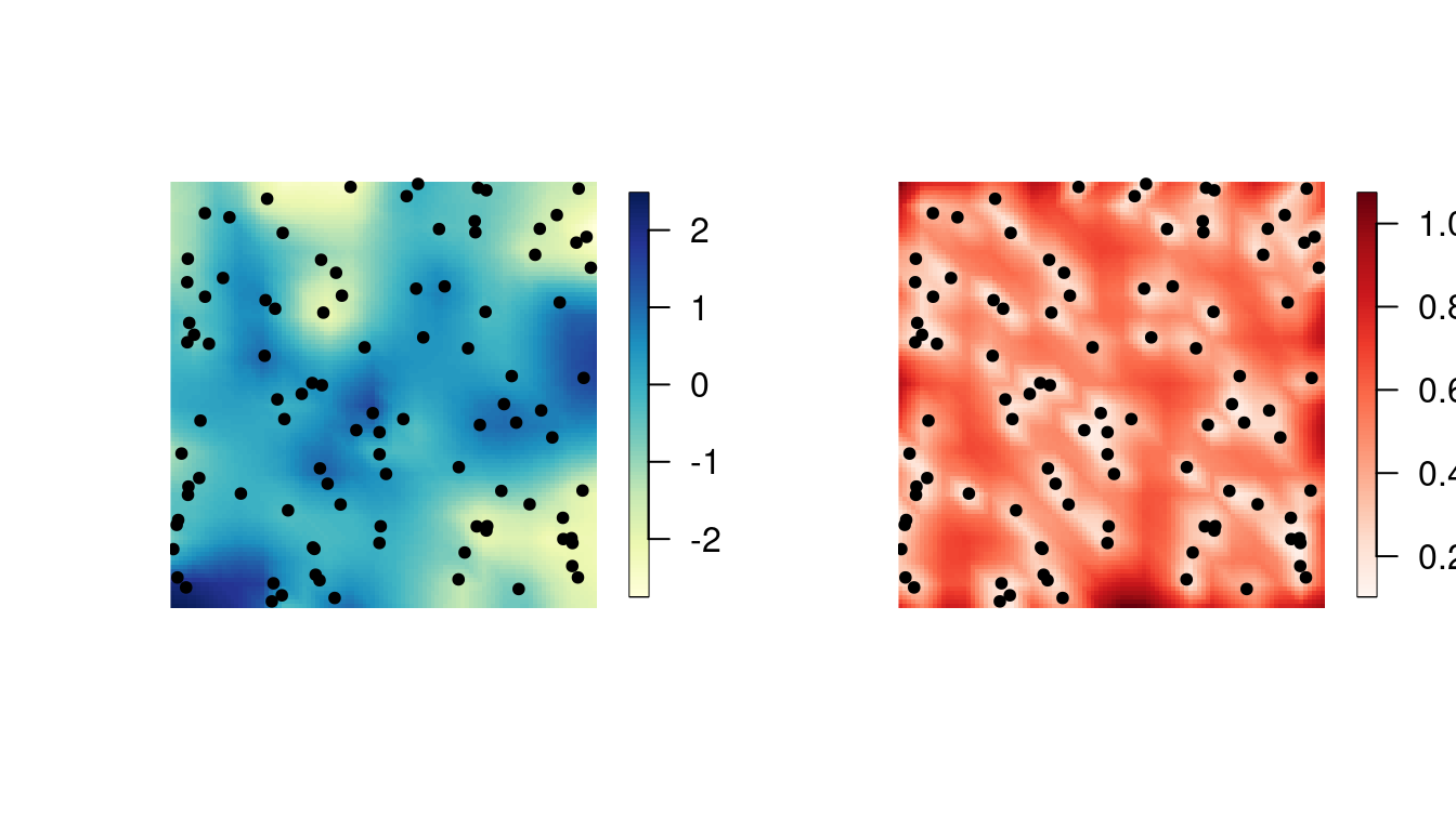
The following figures show the posterior mean and the posterior standard deviations.

proj <- fm_evaluator(mesh, dims = c(100, 100))
cmap <- colorRampPalette(brewer.pal(9, "YlGnBu"))(100)

sd.post <- excursions.variances(Q = Q.post, max.threads = 2)^0.5
cmap.sd <- colorRampPalette(brewer.pal(9, "Reds"))(100)

par(mfrow=c(1,2))
image.plot(proj$x, proj$y, fm_evaluate(proj, field = mu.post), 
           col = cmap, axes = FALSE,
  xlab = "", ylab = "", asp = 1)
points(obs.loc[, 1], obs.loc[, 2], pch = 20)
image.plot(proj$x, proj$y, fm_evaluate(proj, field = sd.post), 
           col = cmap.sd, axes = FALSE,
  xlab = "", ylab = "", asp = 1)
points(obs.loc[, 1], obs.loc[, 2], pch = 20)

Excursion sets and contour credible regions

The main function for computing excursion sets and contour credible regions is excursions. A typical call to the function looks like

res.exc <-  excursions(mu = mu.post, Q = Q.post, alpha = 0.1, type = '>',
                       u = 0, F.limit = 1)

Here, mu and Q are the mean vector and precision matrix for the joint distribution of the Gaussian vector x. The arguments alpha, u, and type are used to specify what type of excursion set that should be computed: alpha is the error probability, u is the excursion or contour level, and type determines what type of region that is considered: ‘>’ for positive excursion regions, ‘<’ for negative excursion regions, ‘!=’ for contour avoiding regions, and ‘=’ for contour credibility regions. Thus, the call above computes the excursion set $E_{{0,0.1}}^{{+}}$ as introduced in Definitions and computational methodology.

The argument F.limit is used to specify when to stop the computation of the excursion function. In this case with F.limit=1, all values of ${\boldsymbol{\mathrm{F}}}_u^+$ are computed, but the computation time can be reduced by decreasing the value of F.limit.

The function has the EB method as default strategy for handling the possible latent Gaussian structure. In the simulated example, the likelihood is Gaussian and the parameters are assumed to be known, so the EB method is exact. The QC method can be used instead by specifying method='QC'. In this case, the argument rho should be used to also provide a vector with point-wise marginal probabilities: $P(x_i>u)$ for positive excursions and contour regions, and $P(x_i<u)$ for negative excursions. In the situation when $\pi({\boldsymbol{\mathrm{x}}}|{\boldsymbol{\mathrm{Y}}},{\boldsymbol{\mathrm{\theta}}})$ is Gaussian but $\pi({\boldsymbol{\mathrm{x}}}|{\boldsymbol{\mathrm{Y}}})$ is not, the marginal probabilities should be calculated under the distribution $\pi({\boldsymbol{\mathrm{x}}}|{\boldsymbol{\mathrm{Y}}})$ and mu and Q should be chosen as the mean and precision for the distribution $\pi({\boldsymbol{\mathrm{x}}}|{\boldsymbol{\mathrm{Y}}},\hat{{\boldsymbol{\mathrm{\theta}}}})$ where $\hat{{\boldsymbol{\mathrm{\theta}}}}$ is the MAP or ML estimate of the parameters.

The function has a version excursions.inla used to analyze outputs of INLA, which is described further in the INLA interface vignette.

The function excursions.mc can be used to post-process Monte Carlo model simulations in order to compute excursion sets and credible regions. For this function, the model is not specified explicitly. Instead a $d \times N$ matrix X containing $N$ Monte Carlo simulations of the $d$ dimensional process of interest is provided. A basic call to the function looks like

excursions.mc(X, u, type)

where u again determines the level of interest and type defines the type of set that should be computed. It is important to note that this function does all computations purely based on the Monte Carlo samples that are provided, and it does not use any of the computational methods based on sequential importance sampling for Gaussian integrals that the is the basis for the previous methods. This means that this function in one sense is more general as X can be samples from any model, not necessarily a latent Gaussian model. The price that has to be payed for this generality is that the only way of increasing the accuracy of the results is to increase the number of Monte Carlo samples that are provided to the function.

Analysis of contour maps

The main function for analysis of contour maps is contourmap. A basic call to the function looks like

res.con <- contourmap(mu = mu.post, Q = Q.post, 
                      n.levels = 4, alpha = 0.1, 
                      compute = list(F = TRUE, measures = c("P0")))

Here, mu is again the mean value and Q is the precision matrix of the model. The parameter n.levels sets the number of contours that should be used in the contour map, and these are spaced equidistant in the range of mu by default. Other types of contour maps can be obtained using the type argument. For manual specification of the levels, the levels argument can be used instead. By default, the function computes the specified contour map but no quality measures and it does not compute the contour map function. If quality measures should be computed, this is specified using the compute argument. This argument is also used to decide whether the contour map function $F$ should be computed.

As for excursions, this function comes in two other versions depending on the form of the input: contourmap.inla for model specification using an INLA object, or contourmap.mc for model specification using Monte Carlo simulations of the model. The model specification using these functions is identical to that in the corresponding excursions functions. See the INLA interface vignette for examples using contourmap.inla.

Continuous domain interpretations

A common scenario is that the input used in contourmap or excursions represents the value of the model at some discrete locations in a continuous domain of interest. In this case, the function continuous can be used to interpolate the discretely computed values by assuming monotonicity of the random field in between the discrete computation locations, as discussed in Definitions and computational methodology. A typical calls to the function looks like

sets.exc <- continuous(ex = res.exc, geometry = mesh, alpha = 0.1)

Here ex is the result of the call to contourmap or excursions and alpha is the error probability of interest for the excursion set or credible region computation. The argument geometry specifies the geometric configuration of the values in input ex, either as a general triangulation geometry or as a lattice. A lattice can be specified as an object of the form list(x, y) where x and y are vectors, or as list(loc, dims) where loc is a two-column matrix of coordinates, and is the lattice size vector. If INLA is used, the lattice can also be specified as an fm_lattice_2d object. In all cases, the input is treated topologically as a lattice with lattice boxes that are assumed convex. A triangulation geometry is specified as an fm_mesh_2d object. Finally, an argument output can be used to specify what type of object should be generated. The options are currently sp which gives a SpatialPolygons object, and inla which gives an fm_segm object.

Simultaneous confidence bands

The function simconf can be used for calculating simultaneous confidence bands for a Gaussian process $X(s)$. A basic call to the function looks like

simconf(alpha, mu, Q)

where alpha is the coverage probability, mu is the mean value vector for the process, and Q is the precision matrix for the process. The function has a few optional arguments similar to those of excursions, all listed in the documentation of the function. The function returns upper and lower limits for both pointwise and simultaneous confidence bands.

As for excursions and contourmap, there is also a version of simconf that can be used to analyze INLA models (simconf.inla) and a version that can analyze Monte Carlo samples (simconf.mc). Furthermore, there is a version simconf.mixture which is used to compute simultaneous confidence regions for Gaussian mixture models with a joint distribution on the form $$\pi(x) = \sum_{k=1}^K w_k N(\mu_k, Q_k^{-1}).$$ This particular function was used to analyze the models in (Bolin et al. 2015) and (Guttorp et al. 2014), but is also used internally by simconf.inla.

Gaussian integrals

Among the utility functions in the package, the function gaussint can be especially useful also in a larger context. It contains the implementation of the sequential importance sampling method for computing Gaussian integrals, described in Definitions and computational methodology. This function has two features that separates it from many other functions for computing Gaussian integrals: Firstly it is based on the precision matrix of the Gaussian distribution, and sparsity of this matrix can be utilized to decrease computation time. Secondly, the integration can be stopped as soon as the value of the integral in the sequential integration goes below some given value $1-\alpha$. If one only is interested in the exact value of the integral given that it is larger than some value $1-\alpha$, this option can save a lot of computation time.

A basic call to the function looks like

gaussint(mu, Q, a, b)

where mu is the mean value vector, Q is the precision matrix, a is a vector of the lower limits in the integral, and b contains the upper integration limits. If the Cholesky factor of Q is known beforehand, this can be supplied to the function using the Q.chol argument. An argument alpha is used to set the computational $1-\alpha$ limit for the integral. The function returns an estimate of the integral as well as an error estimate. If the error estimate is too high, the precision can be increased by increasing the n.iter argument of the function.

Plotting

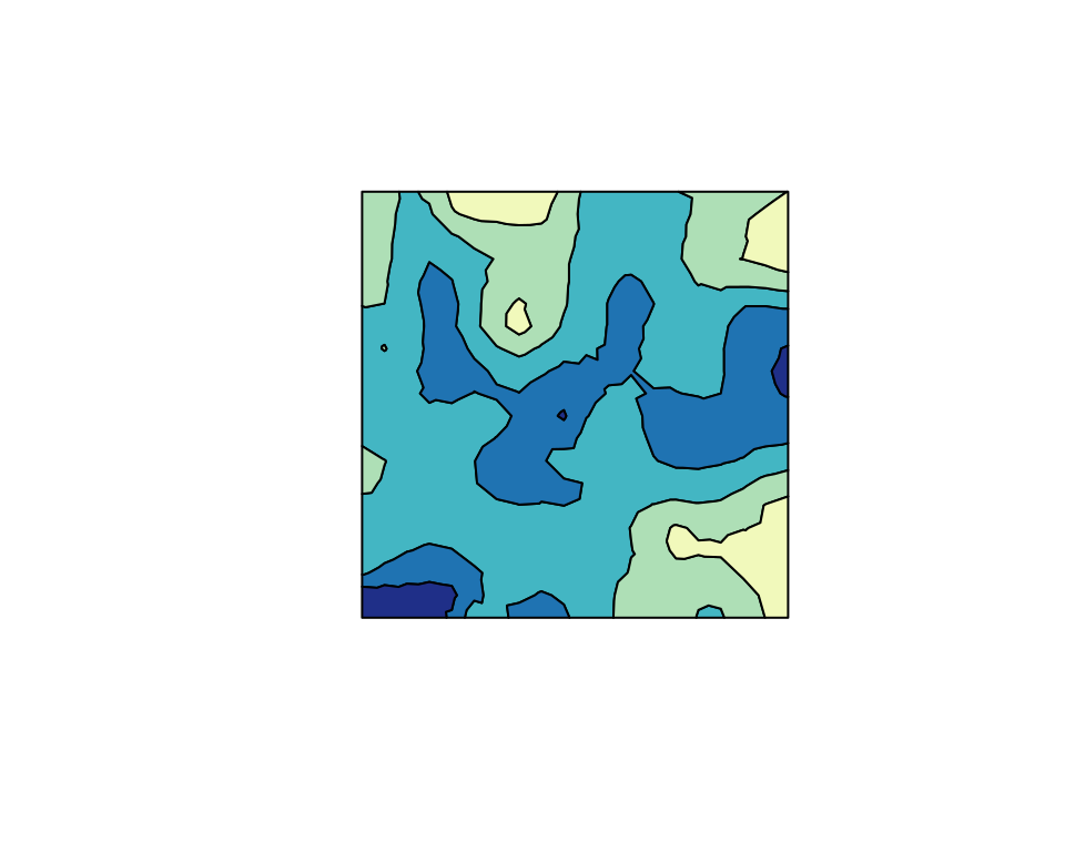
The excursions package contains various functions that are useful for visualization. The function tricontourmap can be used for visualization of contour maps computed on triangulated meshes. The following code plots the posterior mean using the contour map we previously computed.

set.sc <- tricontourmap(mesh, 
                        z = mu.post, 
                        levels = res.con$u)
plot(set.sc$map, col = contourmap.colors(res.con, col = cmap))

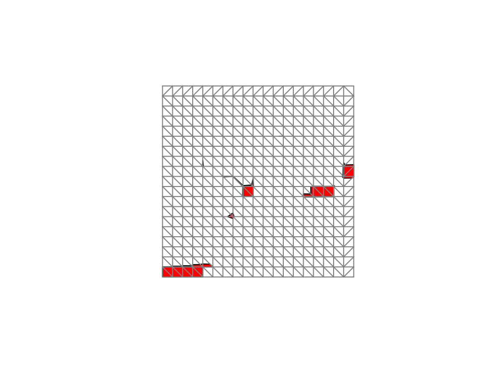
Here contourmap.colors is used to find appropriate colors for each set in the contour map, based on the color map cmap that was defined using the RColorBrewer package. The estimated excursion set can be visualized as

plot(sets.exc$M["1"], col = "red", 
     xlim = range(mesh$loc[,1]),
     ylim = range(mesh$loc[,2]))
plot(mesh, vertex.color = rgb(0.5, 0.5, 0.5), 
     draw.segments = FALSE,
     edge.color = rgb(0.5, 0.5, 0.5), 
     add = TRUE)

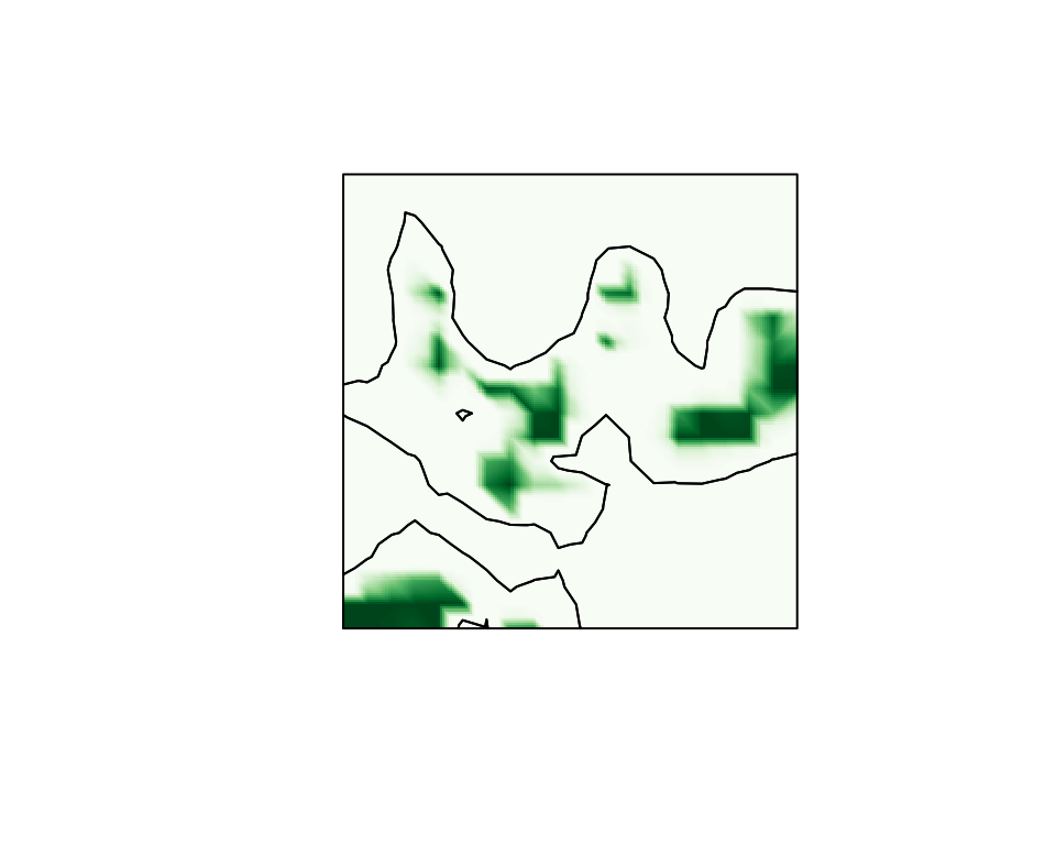
The second plot command adds the mesh to the plot so that we can see how the set is interpolated by the continuous function. Finally, the interpolated excursion function $F_u^+({\boldsymbol{\mathrm{s}}})$, can be plotted easily using the fm_evaluator function from the INLA package.

cmap.F <- colorRampPalette(brewer.pal(9, "Greens"))(100)
proj <- fm_evaluator(sets.exc$F.geometry, dims = c(200, 200))
image(proj$x, proj$y, fm_evaluate(proj, field = sets.exc$F),
      col = cmap.F, axes = FALSE, xlab = "", ylab = "", asp = 1)
con <- tricontourmap(mesh, z = mu.post, levels = 0)
plot(con$map, add = TRUE)

The final two lines computes the level zero contour curve and plots it in the same figure as the interpolated excursion function.

References

Bolin, David, Peter Guttorp, Alex Januzzi, Daniel Jones, Marie Novak, Harry Podschwit, Lee Richardson, Aila Särkkä, Colin Sowder, and Aaron Zimmerman. 2015. “Statistical Prediction of Global Sea Level from Global Temperature.” Statistica Sinica 25: 351–67. https://doi.org/10.5705/ss.2013.222w.

Guttorp, Peter, Alex Januzzi, Marie Novak, Harry Podschwit, Lee Richardson, Colin D Sowder, Aaron Zimmerman, David Bolin, and Aila Särkkä. 2014. “Assessing the Uncertainty in Projecting Local Mean Sea Level from Global Temperature.” Journal of Applied Meteorology and Climatology 53 (9): 2163–70. https://doi.org/10.1175/jamc-d-13-0308.1.

Lindgren, Finn, Håvard Rue, and Johan Lindström. 2011. “An Explicit Link Between Gaussian Fields and Gaussian Markov Random Fields: The Stochastic Partial Differential Equation Approach (with Discussion).” Journal of the Royal Statistical Society B 73: 423–98. https://doi.org/10.1111/j.1467-9868.2011.00777.x.

Lindgren, F., and H. Rue. 2015. “Bayesian Spatial and Spatiotemporal Modelling with .” Journal of Statistical Software 63 (19). https://doi.org/10.18637/jss.v063.i19.