Excursion Sets and Contour Credibility Regions for Random Fields

excursions is one of the main functions in the package with the same name. For an introduction to the package, see excursions-package(). The function is used for calculating excursion sets, contour credible regions, and contour avoiding sets for latent Gaussian models. Details on the function and the package are given in the sections below.

Usage

excursions(
  alpha,
  u,
  mu,
  Q,
  type,
  n.iter = 10000,
  Q.chol,
  F.limit,
  vars,
  rho,
  reo,
  method = "EB",
  ind,
  max.size,
  verbose = 0,
  max.threads = 0,
  seed,
  prune.ind = FALSE
)

Arguments

alpha

Error probability for the excursion set.

u

Excursion or contour level.

mu

Expectation vector.

Q

Precision matrix.

type

Type of region:

'>': positive excursion region
'<': negative excursion region
'!=': contour avoiding region
'=': contour credibility region

n.iter

Number or iterations in the MC sampler that is used for approximating probabilities. The default value is 10000.

Q.chol

The Cholesky factor of the precision matrix (optional).

F.limit

The limit value for the computation of the F function. F is set to NA for all nodes where F<1-F.limit. Default is F.limit = alpha.

vars

Precomputed marginal variances (optional).

rho

Marginal excursion probabilities (optional). For contour regions, provide \(P(X>u)\).

reo

Reordering (optional).

method

Method for handeling the latent Gaussian structure:

'EB': Empirical Bayes (default)
'QC': Quantile correction, rho must be provided if QC is used.

ind

Indices of the nodes that should be analysed (optional).

max.size

Maximum number of nodes to include in the set of interest (optional).

verbose

Set to TRUE for verbose mode (optional).

max.threads

Decides the number of threads the program can use. Set to 0 for using the maximum number of threads allowed by the system (default).

seed

Random seed (optional).

prune.ind

If TRUE and ind is supplied, then the result object is pruned to contain only the active nodes specified by ind.

Value

excursions returns an object of class "excurobj" with the following elements

E: Excursion set, contour credible region, or contour avoiding set
G: Contour map set. \(G=1\) for all nodes where the \(mu > u\).
M: Contour avoiding set. \(M=-1\) for all non-significant nodes. \(M=0\) for nodes where the process is significantly below u and \(M=1\) for all nodes where the field is significantly above u. Which values that should be present depends on what type of set that is calculated.
F: The excursion function corresponding to the set E calculated or values up to F.limit
rho: Marginal excursion probabilities
mean: The mean mu.
vars: Marginal variances.
meta: A list containing various information about the calculation.

Details

The estimation of the region is done using sequential importance sampling with n.iter samples. The procedure requires computing the marginal variances of the field, which should be supplied if available. If not, they are computed using the Cholesky factor of the precision matrix. The cost of this step can therefore be reduced by supplying the Cholesky factor if it is available.

The latent structure in the latent Gaussian model can be handled in several different ways. The default strategy is the EB method, which is exact for problems with Gaussian posterior distributions. For problems with non-Gaussian posteriors, the QC method can be used for improved results. In order to use the QC method, the true marginal excursion probabilities must be supplied using the argument rho. Other more complicated methods for handling non-Gaussian posteriors must be implemented manually unless INLA is used to fit the model. If the model is fitted using INLA, the method excursions.inla can be used. See the Package section for further details about the different options.

References

Bolin, D. and Lindgren, F. (2015) Excursion and contour uncertainty regions for latent Gaussian models, JRSS-series B, vol 77, no 1, pp 85-106.

Bolin, D. and Lindgren, F. (2018), Calculating Probabilistic Excursion Sets and Related Quantities Using excursions, Journal of Statistical Software, vol 86, no 1, pp 1-20.

Author

David Bolin davidbolin@gmail.com and Finn Lindgren finn.lindgren@gmail.com

Examples

## Create a tridiagonal precision matrix
n <- 21
Q.x <- sparseMatrix(
  i = c(1:n, 2:n), j = c(1:n, 1:(n - 1)), x = c(rep(1, n), rep(-0.1, n - 1)),
  dims = c(n, n), symmetric = TRUE
)
## Set the mean value function
mu.x <- seq(-5, 5, length = n)

## calculate the level 0 positive excursion function
res.x <- excursions(
  alpha = 1, u = 0, mu = mu.x, Q = Q.x,
  type = ">", verbose = 1, max.threads = 2
)
#> Calculate marginals
#> Calculate permutation
#> Calculate limits

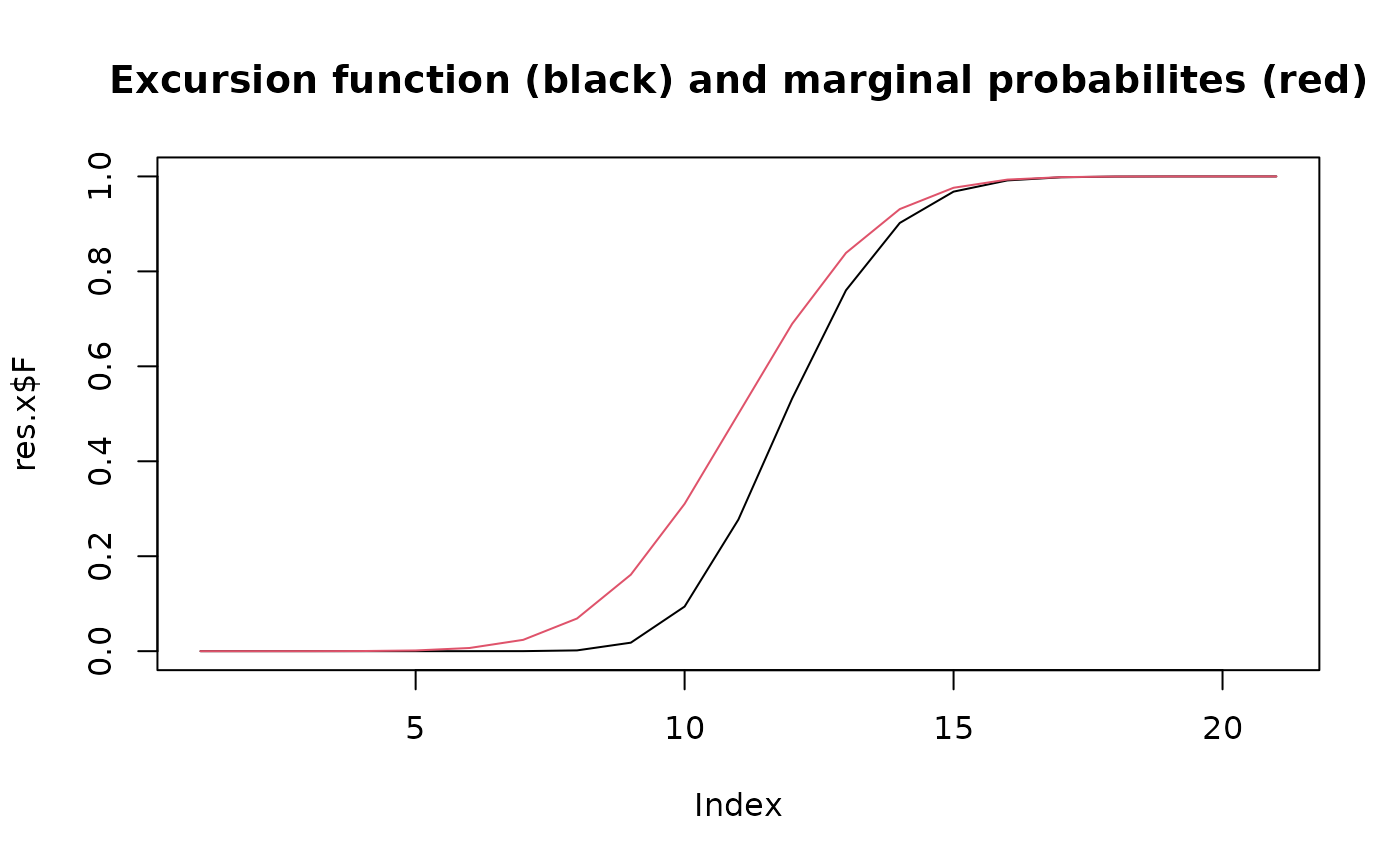
## Plot the excursion function and the marginal excursion probabilities
plot(res.x$F,
  type = "l",
  main = "Excursion function (black) and marginal probabilites (red)"
)
lines(res.x$rho, col = 2)