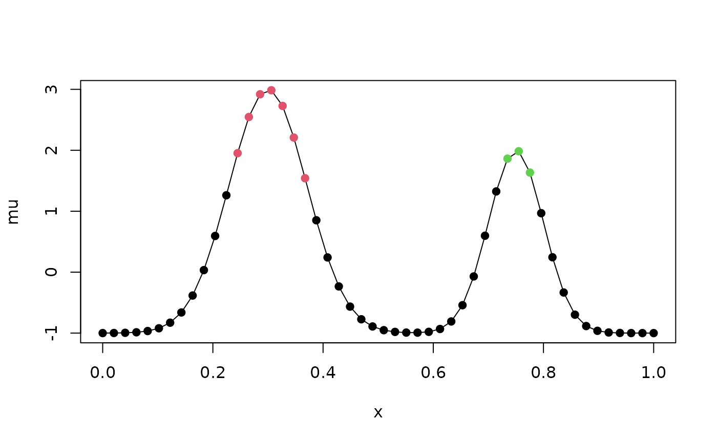
Connected Excursion Regions for Gaussian Random Fields

excursions.regions computes connected (contiguous) regions where a Gaussian random field jointly exceeds a level with high probability. The first region is the largest connected region \(D\) that is found with \(P(X(s) > u, s \in D) \geq 1 - \alpha\). The nodes of the region are then removed, and the search is repeated for the second largest region, and so on. Each region individually satisfies the probability requirement, and the regions do not overlap.

Usage

excursions.regions(
  alpha,
  u,
  mu,
  Q,
  type,
  graph,
  n.iter = 20000,
  vars,
  rho,
  method = "EB",
  ind,
  max.regions = Inf,
  min.size = 1,
  growth = c("bound", "rho"),
  n.starts = 10,
  min.prominence = 0,
  max.threads = 0,
  seed,
  verbose = 0,
  tol = NULL,
  size.tol = 0.001
)

Arguments

alpha

Error probability for each region.

u

Excursion level.

mu

Expectation vector.

Q

Precision matrix.

type

Type of region, '>' for positive excursion regions and '<' for negative excursion regions.

graph

The neighbourhood graph that defines which nodes are connected, given as a symmetric sparse matrix where the non-zero off-diagonal elements are the edges, or as an fm_mesh_2d object, in which case the vertex graph of the mesh is used. The default is the graph of the non-zero elements of Q.

n.iter

Number or iterations in the MC sampler that is used for approximating probabilities. The default value is 20000. If size.tol or tol is given, this is the maximal number of iterations.

vars

Precomputed marginal variances (optional).

rho

Marginal excursion probabilities (optional).

method

Method for handling the latent Gaussian structure:

'EB': Empirical Bayes (default)
'QC': Quantile correction, rho must be provided if QC is used.

ind

Indices of the nodes that can be included in the regions (optional).

max.regions

The maximum number of regions to compute. The default computes all regions.

min.size

The minimum number of nodes of a region. Regions with fewer nodes are not computed.

growth

How the regions are grown from the node with the largest marginal probability:

'bound': The region grows by the neighbour that decreases a lower bound of the joint probability the least (default). This prefers nodes that are strongly correlated with the region.
'rho': The region grows by the neighbour with the largest marginal excursion probability.

n.starts

The maximum number of start points for growing a region in each connected component. The start points are the local maxima of the marginal excursion probabilities in the component, largest first, and the largest region over the start points is kept. Local maxima in the largest region found so far are skipped, and do not count towards n.starts.

min.prominence

The minimum prominence of a local maximum for it to be used as a start point, on the standardised scale \((\mu - u)/\sigma\). The prominence is how far the standardised margin must decrease from the maximum before a higher maximum can be reached, so small values remove maxima that are caused by noise in the mean. The largest maximum of each component is always used.

max.threads

The number of threads that the program can use. The default, 0, uses the default number of threads of OpenMP.

seed

Random seed (optional).

verbose

Set to TRUE for verbose mode (optional).

tol

Target for the estimated errors of the joint probabilities of the regions where they pass 1 - alpha (optional). If tol is given, the number of iterations is chosen adaptively, using at most n.iter iterations, see gaussint(). It takes precedence over size.tol.

size.tol

Target for the estimated Monte Carlo error of the size of each region, relative to the size, when it is grown, see excursions(). The default is 0.001. It is not used if tol is given.

Value

excursions.regions returns a list with the elements

regions: A list with the node indices of the regions, largest first.
P: The estimated joint excursion probability of each region.
P.err: The Monte Carlo standard errors of P.
labels: A vector with the region of each node, where 0 means that the node is not in a region.
E: The largest region, as an indicator vector.
F: The excursion functions of the regions, as a sparse matrix with one column for each region. See the details.
rho: Marginal excursion probabilities.
mean: The mean mu.
vars: Marginal variances.
meta: A list containing various information about the calculation.

Details

A connected region can only contain nodes with marginal excursion probability at least \(1-\alpha\), so the search is done within each connected component of these nodes. In each component, a region is grown from a start point, which gives a sequence of connected regions where each region contains the previous one. The joint excursion probabilities of all regions in the sequence are computed with one run of the sequential importance sampler, and the largest region with probability at least \(1-\alpha\) is kept. The start points are the local maxima of the marginal excursion probabilities in the component, computed on the standardised scale \((\mu - u)/\sigma\) to avoid ties for probabilities close to one. Up to n.starts local maxima are tried, largest first, since the largest maximum does not always give the largest region, and the largest region over the start points is kept. Local maxima in the largest region found so far are skipped. Finding the largest connected region is a hard combinatorial problem, and the region that is found is not guaranteed to be the largest one. The joint probability of each returned region is however computed as in excursions().

With growth = 'bound', the node added in each step is the one that decreases the Hunter lower bound of the joint probability the least. This uses the pairwise failure probabilities of neighbouring nodes, which are computed from the marginal variances and the covariances between neighbours. These are obtained from the selected inverse of Q. Edges of graph that are not in the sparsity pattern of the Cholesky factor of Q are used for connectivity, but not for the bound.

Each region has an excursion function, which is given for the nodes of the region and for their neighbours. A region \(R\) is the largest set in a sequence of growing connected sets, and the excursion function at a node of the region is the joint excursion probability of the smallest set in the sequence that contains the node, so the region is the set where the excursion function is at least \(1-\alpha\). At a neighbour \(j\) of the region, the excursion function is the joint excursion probability of \(R\) together with \(j\). These are computed for all neighbours with one run of the sampler, and if a neighbour that could be in the region has a probability of at least \(1-\alpha\), it is added to the region. The excursion function is zero at the nodes of the other regions and at all other nodes, and it is used by continuous() to compute continuous domain regions.

After a region is found, its nodes are removed, and the remaining nodes of its component are split into new components that are searched in the same way. Regions grown from the other start points of the component are reused in the new components if they do not overlap the removed region, so these start points do not need to be computed again. Every node with marginal excursion probability at least \(1-\alpha\) is a region of size one, so without max.regions or min.size, the regions cover all such nodes.

The regions are computed jointly for all nodes in mu, with the other nodes integrated out, so each start point requires a Cholesky factorisation of Q. Components with a single node are computed directly from the marginal probabilities.

References

Bolin, D. and Lindgren, F. (2015) Excursion and contour uncertainty regions for latent Gaussian models, JRSS-series B, vol 77, no 1, pp 85-106.

Author

David Bolin davidbolin@gmail.com

Examples

## A field on a line with two bumps
n <- 50
Q <- sparseMatrix(
  i = c(1:n, 2:n), j = c(1:n, 1:(n - 1)),
  x = c(1, rep(1 + 0.9^2, n - 2), 1, rep(-0.9, n - 1)) / (1 - 0.9^2),
  dims = c(n, n), symmetric = TRUE
)
x <- seq(0, 1, length.out = n)
mu <- 4 * exp(-(x - 0.3)^2 / 0.01) + 3 * exp(-(x - 0.75)^2 / 0.005) - 1
res <- excursions.regions(
  alpha = 0.1, u = 0, mu = mu, Q = Q, type = ">",
  min.size = 3, seed = 1, max.threads = 1
)
res$regions
#> [[1]]
#> [1] 13 14 15 16 17 18 19
#> 
#> [[2]]
#> [1] 37 38 39
#> 
res$P
#> [1] 0.9137107 0.9289390
plot(x, mu, type = "l")
points(x, mu, col = res$labels + 1, pch = 19)