VAR(1) Bivariate Model in ngme2

Introduction

The Vector Autoregressive model of order 1 (VAR(1)) extends the univariate AR(1) to a bivariate (or multivariate) setting. At each time step the state vector depends linearly on the previous state:

$\mathbf{y}_t = A\,\mathbf{y}_{t-1} + \boldsymbol{\varepsilon}_t, \qquad t = 2, \ldots, T$

where $\mathbf{y}_t = (y_{1,t}, y_{2,t})^\top \in \mathbb{R}^2$ and $A$ is a $2\times 2$ VAR coefficient matrix. For the process to be stationary, all eigenvalues of $A$ must lie strictly inside the unit circle, i.e. $\rho(A) < 1$ .

The ngme2 package provides var1(), which:

Guarantees stationarity via the Cayley reparameterization (see below).
Supports non-Gaussian innovations $\boldsymbol{\varepsilon}_t$ (NIG, GAL, normal).
Integrates seamlessly with the rest of ngme2: fixed effects, measurement noise, prediction.

Model Specification

Precision matrix

Multiplying both sides of the VAR(1) equation by the inverse factor gives the precision structure. Define the $T\times T$ matrices

$G = I_T, \qquad C_{t,t-1} = -1 \text{ (sub-diagonal)}, \text{ all other entries zero.}$

The $2T\times 2T$ precision matrix of $(\mathbf{y}_1,\ldots,\mathbf{y}_T)$ is

$K(A) = M_0 + a_{11}M_{11} + a_{22}M_{22} + a_{12}M_{12} + a_{21}M_{21},$

where:

Matrix	Block structure	Encodes
$M_0 = \mathrm{blkdiag}(G,G)$	$2T\times 2T$ identity	Base
$M_{11} = \mathrm{blkdiag}(C, 0)$	top-left $T\times T$ block	Own-lag $y_1 \leftarrow y_1$
$M_{22} = \mathrm{blkdiag}(0, C)$	bottom-right $T\times T$ block	Own-lag $y_2 \leftarrow y_2$
$M_{12}$	top-right $T\times T$ block	Cross-lag $y_1 \leftarrow y_2$
$M_{21}$	bottom-left $T\times T$ block	Cross-lag $y_2 \leftarrow y_1$

The sub-diagonal of each block carries the coefficient $-a_{ij}$ (sign convention from the $K\mathbf{y}=\boldsymbol\varepsilon$ formulation).

Cayley reparameterization

Directly optimizing $A$ does not guarantee stationarity: $|a_{ii}| < 1$ for each element is necessary but not sufficient (e.g. $A = \bigl[\begin{smallmatrix}0.9 & 0.9\\ 0.9 & 0.9 \end{smallmatrix}\bigr]$ has $\rho(A)\approx 1.27$ ).

var1() uses four unconstrained parameters $\theta = (p_1, p_2, p_3, p_4)$ and the Cayley transform to produce any stationary $2\times 2$ matrix:

$J = \begin{pmatrix} 0 & p_1 \\ -p_1 & 0 \end{pmatrix},\quad L = \begin{pmatrix} p_2 & 0 \\ p_3 & p_4 \end{pmatrix},\quad R = LL^\top + \varepsilon I_2$

$S = J - R, \qquad A = (I_2 + S)(I_2 - S)^{-1}.$

Why does this guarantee $\rho(A)<1$ ?

$S + S^\top = J + J^\top - 2R = -2R$ , which is negative definite. Hence every eigenvalue of $S$ has strictly negative real part. The Cayley transform maps matrices with all eigenvalues having $\text{Re}(\lambda) < 0$ to matrices with all eigenvalues inside the unit disk: $|\text{eigenvalue}(A)| < 1$ .

# Helper: Cayley transform given unconstrained params
cayley_to_A <- function(p, eps = 1e-5) {
  J <- matrix(c(0, -p[1], p[1], 0), 2)
  L <- matrix(c(p[2], p[3], 0, p[4]), 2)
  R <- L %*% t(L) + eps * diag(2)
  S <- J - R
  I2 <- diag(2)
  solve(I2 - S, I2 + S)
}

# Verify: 10,000 random unconstrained params always give rho(A) < 1
set.seed(42)
max_sr <- max(replicate(10000, {
  p <- rnorm(4, sd = 3)
  p[2] <- abs(p[2]) + 0.01
  p[4] <- abs(p[4]) + 0.01
  max(abs(eigen(cayley_to_A(p), only.values = TRUE)$values))
}))
cat(sprintf("Maximum spectral radius over 10,000 random draws: %.6f\n", max_sr))
#> Maximum spectral radius over 10,000 random draws: 0.999764

Interpretation of the parameters:

Parameter	Role
$p_1$	rotation (skew-symmetric part of $S$ )
$p_2, p_4$	contraction strength along each axis (diagonal of $L$ )
$p_3$	off-diagonal mixing in the contraction factor

The default $(p_1,p_2,p_3,p_4)=(0,1,0,1)$ gives $A \approx -\varepsilon/(2+\varepsilon)\,I_2 \approx 0$ (effectively no temporal dependence at initialization).

Using `var1()` in ngme2

Function signature

var1(mesh = NULL, p1 = 0, p2 = 1, p3 = 0, p4 = 1)

Argument	Meaning
`mesh`	Integer vector `1:T` (or a 1-D fmesher mesh) defining the time grid
`p1`–`p4`	Starting values for the four Cayley parameters

Data layout

All observations from both series are stacked into a single vector:

y   <- c(y1[1:T], y2[1:T])      # stacked response
idx <- rep(1:T, 2)               # time index
group <- factor(c(rep("y1", T), rep("y2", T)))

Model formula

ngme(
  y ~ 0 + f(idx,
             model = var1(mesh = 1:T),
             group = group,
             noise = noise_nig()),
  data        = data.frame(y, idx, group),
  group       = group,
  family      = noise_normal()
)

Simulation Study

We simulate a VAR(1)-NIG process with a known coefficient matrix, fit the model, and verify parameter recovery.

True parameters

We choose

$A_{\text{true}} = \begin{pmatrix} 0.6 & 0.3 \\ -0.2 & 0.5 \end{pmatrix}, \qquad \rho(A_{\text{true}}) = 0.6$

and invert the Cayley map to obtain the corresponding unconstrained parameters.

# True VAR coefficient matrix
A_true <- matrix(c(0.6, -0.2, 0.3, 0.5), nrow = 2)
cat("A_true:\n")
#> A_true:
print(A_true)
#>      [,1] [,2]
#> [1,]  0.6  0.3
#> [2,] -0.2  0.5
cat("Spectral radius:", max(abs(eigen(A_true)$values)), "\n")
#> Spectral radius: 0.6

# Invert Cayley:  S = (A - I)(A + I)^{-1},  R = (S^T + S)/(-2),  J = S + R
eps <- 1e-5
I2 <- diag(2)
S_inv <- solve(A_true + I2, A_true - I2)
R_inv <- -(S_inv + t(S_inv)) / 2 # positive definite
J_inv <- S_inv + R_inv # skew-symmetric

# Extract unconstrained params
p1_true <- J_inv[1, 2]
L_true <- t(chol(R_inv - eps * I2)) # lower-triangular Cholesky
p2_true <- L_true[1, 1]
p3_true <- L_true[2, 1]
p4_true <- L_true[2, 2]

cat(sprintf(
  "\nUnconstrained params:  p1=%.4f  p2=%.4f  p3=%.4f  p4=%.4f\n",
  p1_true, p2_true, p3_true, p4_true
))
#> 
#> Unconstrained params:  p1=0.2033  p2=0.4685  p3=-0.0868  p4=0.5415

# Verify round-trip
A_check <- cayley_to_A(c(p1_true, p2_true, p3_true, p4_true))
cat("Round-trip error:", max(abs(A_check - A_true)), "\n")
#> Round-trip error: 1.110223e-16

NIG innovation noise with:

mu_true <- 1.0 # skewness
sigma_true <- 1.0 # scale
nu_true <- 1.5 # heavy-tailedness (smaller = heavier tails)
sigma_eps <- 0.3 # measurement noise std

Simulate the process

set.seed(2025)
T <- 400
group <- factor(c(rep("y1", T), rep("y2", T)), levels = c("y1", "y2"))

f_true <- f(
  c(1:T, 1:T),
  model = var1(
    mesh = 1:T,
    p1 = p1_true, p2 = p2_true,
    p3 = p3_true, p4 = p4_true
  ),
  group = group,
  noise = noise_nig(mu = mu_true, sigma = sigma_true, nu = nu_true)
)

W <- simulate(f_true, nsim = 1)[[1]]
Y <- W + rnorm(2 * T, 0, sigma_eps)

cat(
  "Series y1: mean =", round(mean(Y[1:T]), 2),
  "  sd =", round(sd(Y[1:T]), 2), "\n"
)
#> Series y1: mean = 0.16   sd = 1.95
cat(
  "Series y2: mean =", round(mean(Y[(T + 1):(2 * T)]), 2),
  "  sd =", round(sd(Y[(T + 1):(2 * T)]), 2), "\n"
)
#> Series y2: mean = 0.11   sd = 1.62

Visualise the simulated series

df_plot <- data.frame(
  t = rep(1:T, 2),
  y = Y,
  series = rep(c("y1", "y2"), each = T)
)

ggplot(df_plot, aes(t, y, colour = series)) +
  geom_line(linewidth = 0.5, alpha = 0.8) +
  facet_wrap(~series, ncol = 1, scales = "free_y") +
  labs(
    title = "Simulated VAR(1)-NIG bivariate time series",
    x = "Time", y = "Value"
  ) +
  theme_bw() +
  theme(legend.position = "none")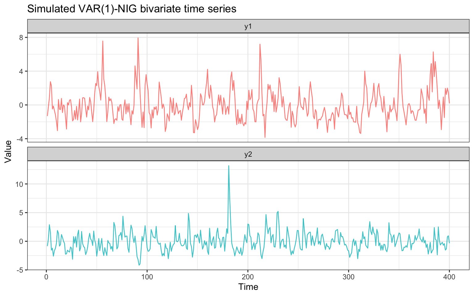

The two series share the same NIG innovation distribution and are cross-correlated through the off-diagonal entries of $A$ .

Cross-correlation check

y1 <- Y[1:T]
y2 <- Y[(T + 1):(2 * T)]
ccf_vals <- ccf(y1, y2, lag.max = 5, plot = FALSE)
cat("CCF at lags -2:+2  (index 4:8 of the acf array):\n")
#> CCF at lags -2:+2  (index 4:8 of the acf array):
print(round(ccf_vals$acf[4:8, , ], 3))
#> [1] -0.286 -0.223  0.003  0.272  0.358
cat("Lags:", ccf_vals$lag[4:8, , ], "\n")
#> Lags: -2 -1 0 1 2

Model Fitting

df <- data.frame(Y = Y, idx = rep(1:T, 2), group = group)

fit <- ngme(
  Y ~ 0 +
    f(idx,
      model = var1(mesh = 1:T),
      name  = "var1field",
      group = group,
      noise = noise_nig()
    ),
  data = df,
  group = df$group,
  family = noise_normal(),
  control_opt = control_opt(
    iterations       = 1000,
    n_parallel_chain = 4,
    seed             = 42
  )
)
#> Starting estimation... 
#> 
#> Starting posterior sampling... 
#> Posterior sampling done! 
#> Average standard deviation of the posterior W:  1.772265 
#> Note:
#>       1. Use ngme_post_samples(..) to access the posterior samples.
#>       2. Use ngme_result(..) to access different latent models.

Summary of estimated model

print(fit)
#> *** Ngme object ***
#> 
#> Fixed effects: 
#>   None
#> 
#> Models: 
#> $var1field
#>   Model type: VAR(1) bivariate model
#>       A (VAR coefficient matrix, Cayley reparameterization):
#>         [[  0.591,   0.287 ],
#>          [  -0.207,   0.520 ]]
#>       spectral radius = 0.6059
#>       unconstrained (p1, p2, p3, p4) =  0.19936,  0.47602, -0.06837,  0.52849
#>   Noise type: NIG
#>   Noise parameters: 
#>       mu = 1.15
#>       sigma = 0.99
#>       nu = 1.81
#> 
#> Measurement noise: 
#>   Noise type: NORMAL
#>   Noise parameters: 
#>       sigma = 0.284

Estimated vs true VAR coefficient matrix

# Extract estimated operator
op_est <- fit$replicates[[1]]$models[["var1field"]]$operator

# Retrieve theta_K from the last iteration (posterior mean over chains)
traj <- attr(fit$replicates[[1]]$models[["var1field"]], "lat_traj")
last_mat <- do.call(cbind, lapply(traj, function(m) m[, ncol(m), drop = FALSE]))
theta_last <- rowMeans(last_mat)[seq_len(4)]

A_est <- op_est$cayley_to_A(theta_last)

cat("True A matrix:\n")
#> True A matrix:
print(round(A_true, 4))
#>      [,1] [,2]
#> [1,]  0.6  0.3
#> [2,] -0.2  0.5
cat("\nEstimated A matrix:\n")
#> 
#> Estimated A matrix:
print(round(A_est, 4))
#>         [,1]   [,2]
#> [1,]  0.5914 0.2874
#> [2,] -0.2068 0.5203
cat("\nMax absolute error:", round(max(abs(A_est - A_true)), 4), "\n")
#> 
#> Max absolute error: 0.0203
cat("True spectral radius:    ", round(max(abs(eigen(A_true)$values)), 4), "\n")
#> True spectral radius:     0.6
cat("Estimated spectral radius:", round(max(abs(eigen(A_est)$values)), 4), "\n")
#> Estimated spectral radius: 0.6059

Noise parameter recovery

# Latent NIG noise (theta_mu on natural scale; theta_sigma/theta_nu log-scale)
noise_lat <- fit$replicates[[1]]$models[["var1field"]]$noise
# Measurement normal noise (theta_sigma log-scale)
noise_meas <- fit$replicates[[1]]$noise

mu_est <- noise_lat$theta_mu
sigma_est <- exp(noise_lat$theta_sigma)
nu_est <- exp(noise_lat$theta_nu)
sigma_eps_est <- exp(noise_meas$theta_sigma)

cat("Parameter  |  True  |  Estimated\n")
#> Parameter  |  True  |  Estimated
cat("-----------|--------|----------\n")
#> -----------|--------|----------
cat(sprintf("mu         |  %.2f  |  %.4f\n", mu_true, mu_est))
#> mu         |  1.00  |  1.1536
cat(sprintf("sigma      |  %.2f  |  %.4f\n", sigma_true, sigma_est))
#> sigma      |  1.00  |  0.9898
cat(sprintf("nu         |  %.2f  |  %.4f\n", nu_true, nu_est))
#> nu         |  1.50  |  1.8065
cat(sprintf("sigma_eps  |  %.2f  |  %.4f\n", sigma_eps, sigma_eps_est))
#> sigma_eps  |  0.30  |  0.2843

Convergence trace plots

# Add horizontal lines at true values for operator params
traceplot(fit,
  hline = c(
    p1_true, p2_true, p3_true, p4_true,
    mu_true, sigma_true, nu_true, sigma_eps
  )
)

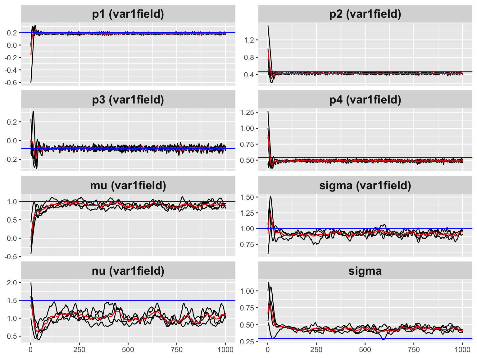
#> Last estimates:
#> $`p1 (var1field)`
#> [1] 0.1993569
#> 
#> $`p2 (var1field)`
#> [1] 0.4760203
#> 
#> $`p3 (var1field)`
#> [1] -0.06837111
#> 
#> $`p4 (var1field)`
#> [1] 0.5284871
#> 
#> $`mu (var1field)`
#> [1] 1.126534
#> 
#> $`sigma (var1field)`
#> [1] 0.9754186
#> 
#> $`nu (var1field)`
#> [1] 1.729008
#> 
#> $sigma
#> [1] 0.3289182

The horizontal dashed lines mark the true parameter values. The chains converge to the correct region within a few hundred iterations.

Gaussian vs Non-Gaussian Noise

To illustrate that the non-Gaussian model is preferred when the data truly contains heavy tails, we fit the same data with Gaussian innovations and compare the log-likelihood.

fit_gauss <- ngme(
  Y ~ 0 +
    f(idx,
      model = var1(mesh = 1:T),
      name  = "var1field",
      group = group,
      noise = noise_normal()
    ),
  data = df,
  group = df$group,
  family = noise_normal(),
  control_opt = control_opt(
    iterations       = 500,
    n_parallel_chain = 4,
    seed             = 42
  )
)
#> Starting estimation... 
#> 
#> Starting posterior sampling... 
#> Posterior sampling done! 
#> Average standard deviation of the posterior W:  1.73551 
#> Note:
#>       1. Use ngme_post_samples(..) to access the posterior samples.
#>       2. Use ngme_result(..) to access different latent models.

ll_nig <- compute_log_like(fit)[[1]]
ll_gauss <- compute_log_like(fit_gauss)[[1]]
cat("NIG model   - log-likelihood:", round(ll_nig, 2), "\n")
#> NIG model   - log-likelihood: 0
cat("Gauss model - log-likelihood:", round(ll_gauss, 2), "\n")
#> Gauss model - log-likelihood: 0

Summary

The var1() function in ngme2 provides a VAR(1) bivariate latent field with:

Guaranteed stationarity at every iteration via the Cayley transform
Non-Gaussian flexibility through NIG / GAL / normal innovation noise
Full integration with ngme2’s MCMC-SGD optimizer, posterior sampling, and traceplots

Key points:

Feature	Detail
Parameterization	4 unconstrained params $(p_1,p_2,p_3,p_4)$
Stationarity	$\rho(A) < 1$ guaranteed by construction
Gradient	Numerical (central differences via `update_all`)
Noise	Single shared NIG/GAL/normal distribution
Data layout	Stacked `y = c(y1, y2)`, `group = factor(...)`

Getting the fitted $A$ matrix

After fitting, recover the VAR coefficient matrix $A$ from the estimated parameters:

op <- fit$replicates[[1]]$models[["var1field"]]$operator
A <- op$cayley_to_A(op$theta_K) # uses the posterior-mean theta_K
rho <- max(abs(eigen(A)$values))
print(A)
cat("Spectral radius:", rho, "\n")