Models with replicates

In this vignette we will introduce the feature of replicates, which allows to include multiple realizations of the stochastic processes that can be included in the different models offered in ngme2.

Description

Consider a stochastic process $\mathbf{W}$ indexed by an index set $\mathbf{I}$ , the idea is to allow the inclusion of replicates of the process in the model.

For example, if one wants to include k realizations of an autoregressive process of order 1 with $n$ observations in the model one can do so in the following way

$\begin{align} X^{(j)}_1 &= \epsilon^{(j)}_1\\ X^{(j)}_i &= \alpha X^{(j)}_{i-1} + \epsilon^{(j)}_i, i = 2, \ \cdots,\ n \end{align}$

where $X^{(j)}_i$ denotes the $i \text{-}th$ observation of $j \text{-}th$ realization of the process for $i = 1, \ \cdots,\ n$ and $j = 1, \ \cdots,\ k$ , with $|\alpha| < 1$ and $\epsilon^{(j)}_1, \ \cdots \ , \epsilon^{(j)}_{n}$ is either i.i.d. NIG or Gaussian noise.

Two approaches for specifying replicates

ngme2 supports two different styles for specifying replicates, each with its own advantages:

Global replicates using the replicate argument in ngme() - applies the same replicate structure to all latent processes in the model
Flexible replicates using the replicate argument in f() - allows individual control over replicate structure for each latent process

Global approach: `replicate` in `ngme()`

The global approach forces every latent process in the model to have the same replicate structure. This is useful when: - You have a simple model with one or few latent processes - All processes should follow the same replicate pattern - You want to ensure consistency across all model components - You have many replicates: The estimation process computes gradients for each replicate separately and sums them, which is memory-efficient for large numbers of replicates

Flexible approach: `replicate` in `f()`

The flexible approach allows different latent processes to have different replicate structures. This offers several additional advantages: - Individual control: Each latent process can have its own replicate structure - INLA-style block-diagonalization: Operators are automatically block-diagonalized across replicates - Flexible mesh support: Different meshes can be used for different replicates - Complex models: Multiple latent processes can have different replicate patterns within the same model - Computational efficiency for moderate cases: The estimation process works with block-diagonalized matrices directly, which is more efficient when dimensions and number of replicates are not too large

Mathematical framework

When using the replicate argument in f(), the precision matrix $\mathbf{K}$ is automatically block-diagonalized:

For a generic operator $\mathbf{K} = \theta_1 \mathbf{M}_1 + \theta_2 \mathbf{M}_2 + \ldots$ with $R$ replicates, the resulting structure becomes:

$\mathbf{K}_{\text{replicated}} = \theta_1 \text{bdiag}(\mathbf{M}_{1,1}, \mathbf{M}_{1,2}, \ldots, \mathbf{M}_{1,R}) + \theta_2 \text{bdiag}(\mathbf{M}_{2,1}, \mathbf{M}_{2,2}, \ldots, \mathbf{M}_{2,R}) + \ldots$

Similarly, the observation matrix $\mathbf{A}$ is constructed for each replicate and then block-diagonalized:

$\mathbf{A}_{\text{replicated}} = \text{bdiag}(\mathbf{A}_1, \mathbf{A}_2, \ldots, \mathbf{A}_R)$

Usage

AR(1) model

The following example will show how to use the replicates feature for an AR(1) model using both approaches.

Suppose one has a response variable with $2n$ observations

library(ngme2)
#> This is ngme2 of version 0.7.0
#> - See our homepage: https://davidbolin.github.io/ngme2 for more details.
library(ggplot2)

# creating ar1 process
n <- 500
myar <- ngme2::f(1:n, model="ar1", rho = .75, noise = noise_nig())

W1 <- simulate(myar, seed = 314)[[1]] # simulating one realization of the process
W2 <- simulate(myar, seed = 159)[[1]] # simulating another realization of the process

# Creating the response variable from the process and adding measurement noise
Y <- -3 + c(W1, W2) + rnorm(2 * n, sd = .2)

df <- data.frame(Y, idx = 1:(2 * n), group = rep(1:2, each = n)) # creating the data frame to fit the model later

Note that if both processes are considered as a single one instead of two realizations of the same process, then the first observation of the second realization is assumed to be dependent on the last one of the first process, which might no be desirable in some cases.

Comparison of K matrices

This can be seen in the $\mathbf{K}$ matrix of the model (all the models in the have the same form $K \mathbf{W} = \mathbf{\epsilon}$ ), for instance, consider the following little example to illustrate the difference between treating the data as a single process vs. replicates.

# No replicates: treats as single AR(1) process with 6 time points
no_replicates <- ngme2::f(1:6, model="ar1", rho = .5, noise = noise_normal())

# With replicates in f(): 2 replicates, each with 3 time points
with_replicates_f <- ngme2::f(
  rep(1:3, 2),
  model = "ar1",
  rho = .5,
  replicate = rep(1:2, each = 3),
  noise = noise_normal()
)

# Compare K matrices
cat("K matrix without replicates (6x6 single process):\n")
#> K matrix without replicates (6x6 single process):
print(as.matrix(no_replicates$operator$K))
#>            [,1] [,2] [,3] [,4] [,5] [,6]
#> [1,]  0.8660254  0.0  0.0  0.0  0.0    0
#> [2,] -0.5000000  1.0  0.0  0.0  0.0    0
#> [3,]  0.0000000 -0.5  1.0  0.0  0.0    0
#> [4,]  0.0000000  0.0 -0.5  1.0  0.0    0
#> [5,]  0.0000000  0.0  0.0 -0.5  1.0    0
#> [6,]  0.0000000  0.0  0.0  0.0 -0.5    1

cat("\nK matrix with replicates (3x3 for each replicate, block-diagonal):\n")
#> 
#> K matrix with replicates (3x3 for each replicate, block-diagonal):
print(as.matrix(with_replicates_f$operator$K))
#>            [,1] [,2] [,3]       [,4] [,5] [,6]
#> [1,]  0.8660254  0.0    0  0.0000000  0.0    0
#> [2,] -0.5000000  1.0    0  0.0000000  0.0    0
#> [3,]  0.0000000 -0.5    1  0.0000000  0.0    0
#> [4,]  0.0000000  0.0    0  0.8660254  0.0    0
#> [5,]  0.0000000  0.0    0 -0.5000000  1.0    0
#> [6,]  0.0000000  0.0    0  0.0000000 -0.5    1

Note how in the replicate version, the $\mathbf{K}_{4,3}$ entry is zero, meaning there’s no dependence between the last observation of the first replicate and the first observation of the second replicate.

Model fitting: global vs flexible approach

Global approach (replicate specified in ngme()):

# Global replicate approach
mod_replicates_global <- ngme(
  formula = Y ~ f(
    c(1:n, 1:n),
    model = "ar1",
    noise = noise_nig()
  ),
  replicate = df$group,
  data = df,
  control_opt = control_opt(
    print_check_info = FALSE
  )
)
mod_replicates_global

Flexible approach (replicate specified in f()):

# Flexible replicate approach
mod_replicates_flexible <- ngme(
  formula = Y ~ f(
    rep(1:n, 2),
    model = "ar1",
    replicate = df$group,
    noise = noise_nig()
  ),
  data = df,
  control_opt = control_opt(
    verbose = TRUE,
    print_check_info = FALSE
  )
)
mod_replicates_flexible

The flexible approach provides several benefits: - The replicate structure is defined directly with the latent field - Automatic block-diagonalization of operators and A matrices - Support for different meshes per replicate - Allows different latent processes to have different replicate structures

SPDE Matern model

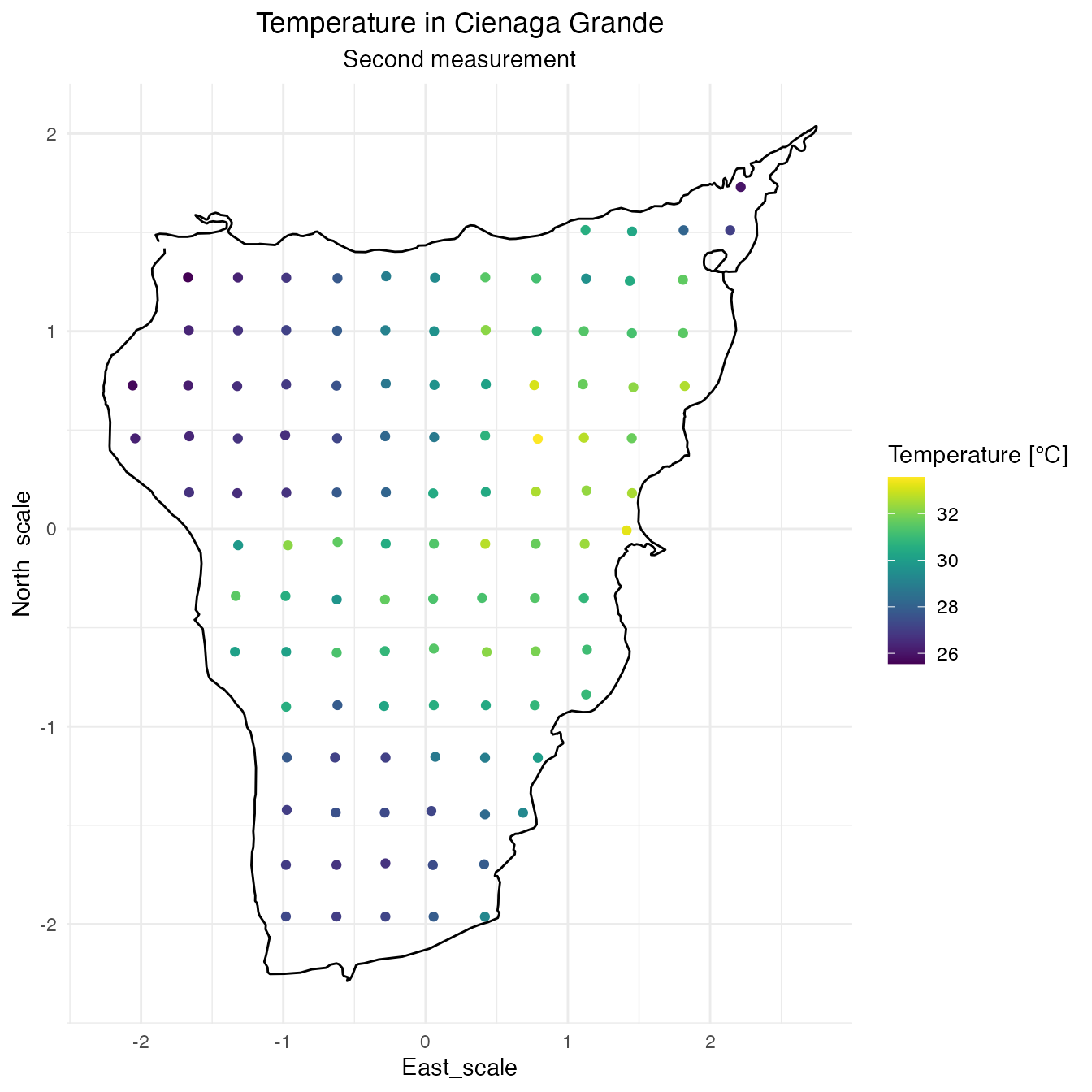
The following data is taken from the swamp of Cienaga Grande in Santa Marta, Colombia. There is a total of 114 locations where some properties of the swamp were measured. Those measurements were taken twice, however there is no information available about their chronological order so this data cannot be treated as spatiotemporal, despite that, the multiple measurements can be treated as replicates.

In this particular case the temperature is the feature that will be modeled.

# library(ngme2)
library(ggplot2)

# reading the data and the boundary of Cienaga Grande
data(cienaga)
data(cienaga.border)
# scale the coords
cienaga.border[, 1] <- (cienaga.border[, 1] - mean(cienaga$East)) / sd(cienaga$East)
cienaga.border[, 2] <- (cienaga.border[, 2] - mean(cienaga$North)) / sd(cienaga$North)
cienaga <- within(cienaga, {
  East_scale <- (East - mean(East)) / sd(East)
  North_scale <- (North - mean(North)) / sd(North)
})

# creating label for the measurement group
cienaga$measurement <- rep(1:2, each = (n <- nrow(cienaga) / 2))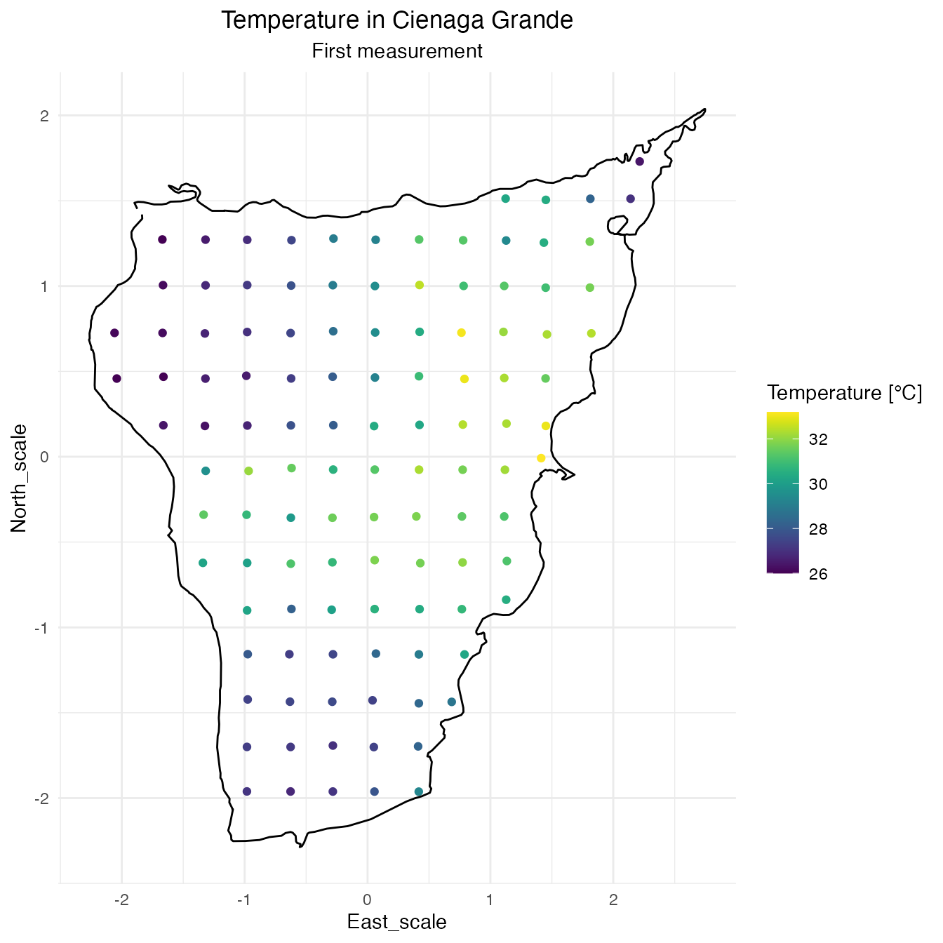

Now we briefly show how to fit the model using both replicate approaches.

# creating the mesh
mesh <- fmesher::fm_mesh_2d(
  loc.domain = cienaga.border,
  max.edge = c(0.4, 1),
  max.n = 500
)
mesh$n
#> [1] 455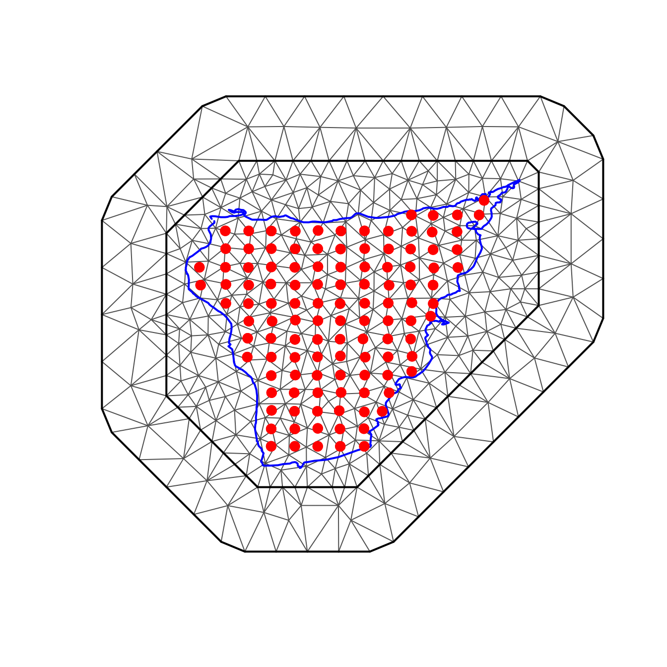

Model fitting: global vs flexible approach for spatial data

Global approach:

# Global replicate approach
fit_global <- ngme(
  formula = temp ~ 1 +
    f(as.matrix(cienaga[, c("East_scale", "North_scale")]), 
      model = "matern", mesh = mesh,
      name = "spde", noise = noise_nig()),
  data = cienaga,
  replicate = cienaga$measurement,
  control_opt = control_opt(
    estimation = TRUE,
    iterations = 500,
    n_slope_check = 10,
    n_parallel_chain = 4,
    print_check_info = FALSE
  ),
  debug = FALSE
)

Flexible approach:

# Flexible replicate approach
fit_flexible <- ngme(
  formula = temp ~ 1 +
    f(as.matrix(cienaga[, c("East_scale", "North_scale")]), 
      model = "matern", 
      mesh = mesh,
      replicate = cienaga$measurement,
      name = "spde", 
      noise = noise_nig()),
  data = cienaga,
  control_opt = control_opt(
    estimation = TRUE,
    iterations = 500,
    n_slope_check = 10,
    n_parallel_chain = 4,
    print_check_info = FALSE
  ),
  debug = FALSE
)

Using different meshes for different replicates

One powerful feature of the flexible approach is the ability to use different meshes for different replicates:

# Create separate meshes for each measurement
coords1 <- as.matrix(cienaga[cienaga$measurement == 1, c("East_scale", "North_scale")])
coords2 <- as.matrix(cienaga[cienaga$measurement == 2, c("East_scale", "North_scale")])

mesh1 <- fmesher::fm_mesh_2d(coords1, cutoff = 0.1)
mesh2 <- fmesher::fm_mesh_2d(coords2, cutoff = 0.1)

# Use different meshes for different replicates (only possible with flexible approach)
fit_multi_mesh <- ngme(
  formula = temp ~ 1 +
    f(as.matrix(cienaga[, c("East_scale", "North_scale")]), 
      model = "matern", 
      mesh = list(mesh1, mesh2),  # List of meshes
      replicate = cienaga$measurement,
      name = "spde", 
      noise = noise_nig()),
  data = cienaga,
  control_opt = control_opt(estimation = FALSE)  # Just for structure
)

Additional examples

RW1 model with replicates

# Random walk model with 3 replicates
base_locations <- 1:10
locations <- rep(base_locations, 3)
replicates <- factor(rep(1:3, each = length(base_locations)))

rw1_replicates <- f(
  map = locations,
  model = "rw1",
  replicate = replicates,
  noise = noise_normal()
)

cat("RW1 with 3 replicates:\n")
#> RW1 with 3 replicates:
cat("- Base length:", length(base_locations), "\n")
#> - Base length: 10
cat("- Number of replicates:", 3, "\n")
#> - Number of replicates: 3
cat("- K matrix size:", paste(dim(rw1_replicates$operator$K), collapse=" x "), "\n")
#> - K matrix size: 30 x 30
cat("- h vector length:", length(rw1_replicates$operator$h), "\n")
#> - h vector length: 30

The K matrix is automatically block-diagonalized:

# Show the structure of the precision matrix for RW1 replicates
K_structure <- as.matrix(rw1_replicates$operator$K)
K_structure[K_structure != 0] <- 1  # Show only the sparsity pattern

# Display first few rows and columns to show block structure
print(K_structure[1:15, 1:15])
#>       [,1] [,2] [,3] [,4] [,5] [,6] [,7] [,8] [,9] [,10] [,11] [,12] [,13]
#>  [1,]    1    0    0    0    0    0    0    0    0     0     0     0     0
#>  [2,]    1    1    0    0    0    0    0    0    0     0     0     0     0
#>  [3,]    0    1    1    0    0    0    0    0    0     0     0     0     0
#>  [4,]    0    0    1    1    0    0    0    0    0     0     0     0     0
#>  [5,]    0    0    0    1    1    0    0    0    0     0     0     0     0
#>  [6,]    0    0    0    0    1    1    0    0    0     0     0     0     0
#>  [7,]    0    0    0    0    0    1    1    0    0     0     0     0     0
#>  [8,]    0    0    0    0    0    0    1    1    0     0     0     0     0
#>  [9,]    0    0    0    0    0    0    0    1    1     0     0     0     0
#> [10,]    0    0    0    0    0    0    0    0    1     1     0     0     0
#> [11,]    0    0    0    0    0    0    0    0    0     0     1     0     0
#> [12,]    0    0    0    0    0    0    0    0    0     0     1     1     0
#> [13,]    0    0    0    0    0    0    0    0    0     0     0     1     1
#> [14,]    0    0    0    0    0    0    0    0    0     0     0     0     1
#> [15,]    0    0    0    0    0    0    0    0    0     0     0     0     0
#>       [,14] [,15]
#>  [1,]     0     0
#>  [2,]     0     0
#>  [3,]     0     0
#>  [4,]     0     0
#>  [5,]     0     0
#>  [6,]     0     0
#>  [7,]     0     0
#>  [8,]     0     0
#>  [9,]     0     0
#> [10,]     0     0
#> [11,]     0     0
#> [12,]     0     0
#> [13,]     0     0
#> [14,]     1     0
#> [15,]     1     1

Summary

ngme2 provides two approaches for handling replicates:

Global approach (`replicate` in `ngme()`)

Applies the same replicate structure to all latent processes
Simple and consistent across the entire model
Suitable for models with uniform replicate patterns

Flexible approach (`replicate` in `f()`)

Individual control: Each latent process can have its own replicate structure
Automatic block-diagonalization: Operators and A matrices are automatically structured for replicates
Flexible mesh support: Different meshes can be used for different replicates
INLA-style implementation: Follows the same approach as INLA for handling replicates
Complex models: Multiple latent processes can have different replicate patterns within the same model

Choose the approach that best fits your modeling needs - use the global approach for simple, uniform replicate structures, and the flexible approach when you need more control or have complex models with varying replicate patterns.

Computational considerations

The two approaches handle the estimation process differently:

Global approach: Computes gradients for each replicate separately and sums them. This is memory-efficient when you have many replicates, as it avoids creating large block-diagonal matrices in memory.
Flexible approach: Creates block-diagonal structures for all replicates together. This is computationally more efficient when the dimension is not too high or when you don’t have too many replicates, as it can take advantage of sparse matrix operations on the entire structure.

Rule of thumb: Use the global approach when you have many replicates (e.g., >50) or high-dimensional problems where memory is a concern. Use the flexible approach for moderate numbers of replicates when you need the additional modeling flexibility or when computational efficiency is important.