Introduction
Metric graph is a class of graphs that are embedded in a metric space. This type of graph can model some specific spatial structures, including road networks, river networks, etc.
In this vignette, we will show how to model a Matern SPDE model on a
metric graph together with the R package
MetricGraph Bolin, Simas, and Wallin (2023b). It
contains functions for working with data and random fields on compact
metric graphs. The main functionality is contained in the
metric_graph class, which is used for specifying metric
graphs, adding data to them, visualization, and other basic functions
that are needed for working with data and random fields on metric
graphs.
To know more about the theory of Matern SPDE model on metric graphs, please refer to Bolin et al. (Bolin, Simas, and Wallin 2023a, 2023c).
library(MetricGraph)
#> This is MetricGraph 1.5.0
#> - See https://davidbolin.github.io/MetricGraph for vignettes and manuals.
#>
#> Attaching package: 'MetricGraph'
#> The following object is masked from 'package:stats':
#>
#>     filter
library(ngme2)
#> This is ngme2 of version 0.9.5
#> - See our homepage: https://davidbolin.github.io/ngme2 for more details.
#>
#> Attaching package: 'ngme2'
#> The following object is masked from 'package:stats':
#>
#>     ar
set.seed(16)
Simulation on a metric graph
First we will build the graph and construct a uniform mesh on each edges.
edge1 <- rbind(c(0, 0), c(1, 0))
edge2 <- rbind(c(0, 0), c(0, 1))
edge3 <- rbind(c(0, 1), c(-1, 1))
theta <- seq(from = pi, to = 3 * pi / 2, length.out = 20)
edge4 <- cbind(sin(theta), 1 + cos(theta))
edges <- list(edge1, edge2, edge3, edge4)
graph <- metric_graph$new(edges = edges)
#> Starting graph creation...
#> LongLat is set to FALSE
#> Creating edges...
#> Setting edge weights...
#> Computing bounding box...
#> Setting up edges
#> Merging close vertices
#> Total construction time: 0.10 secs
#> Creating and updating vertices...
#> Storing the initial graph...
#> Computing the relative positions of the edges...
graph$plot()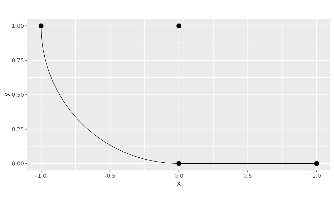
# construct the mesh
graph$build_mesh(h = 0.1)
graph$plot(mesh = TRUE)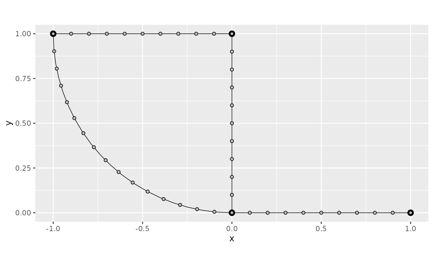
# Refine the mesh and print how many mesh nodes
graph$build_mesh(h = 0.005)
length(graph$mesh$h)
#> [1] 915
Next, we simulation non-Gaussian Matern field with NIG noise using
simulate function.
n.obs <- 1000
edge_number <- sample(1:graph$nE, n.obs, replace = TRUE)
distance_on_edge <- runif(n.obs)
simu_nig <- noise_nig(mu = -10, sigma = 30, nu = 0.5)
matern_graph <- f(
map = cbind(edge_number, distance_on_edge),
model = matern(
kappa = 6,
mesh = graph,
),
noise = simu_nig
)
graph_sim <- simulate(matern_graph, seed = 10)[[1]]
y <- graph_sim + rnorm(length(graph_sim), sd = 0.1)
graph$add_observations(
data = data.frame(
edge_number = edge_number,
distance_on_edge = distance_on_edge,
y = y
),
normalized = TRUE
)
#> Adding observations...
#> Assuming the observations are normalized by the length of the edge.
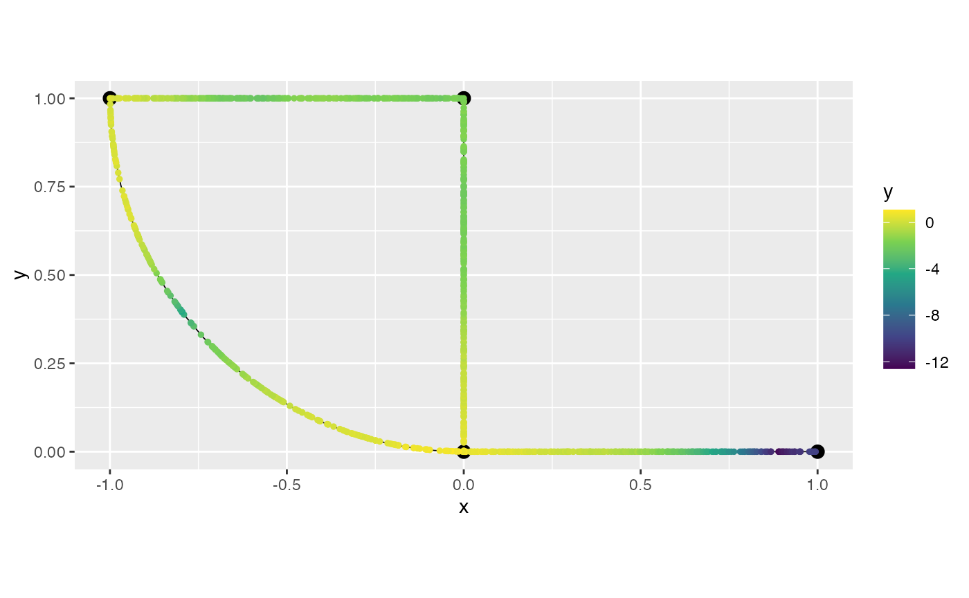
graph$plot(data = "y")
graph$plot(data = "y", plotly = TRUE)
#> Warning: The `plotly` argument of `plot()` is deprecated as of MetricGraph 1.3.0.9000.
#> ℹ Please use the `type` argument instead.
#> ℹ The argument `plotly` was deprecated in favor of the argument `type`.
#> This warning is displayed once every 8 hours.
#> Call `lifecycle::last_lifecycle_warnings()` to see where this warning was
#> generated.
#> Loading required namespace: plotly
Next we estimate the model using ngme2:
fit_nig <- ngme(
  y ~ 0 +
    f(
      map = ~ .edge_number + .distance_on_edge,
      name = "graph",
      model = matern(
        kappa = 6,
        mesh = graph,
      ),
      noise = noise_nig()
    ),
  data = graph$get_data(),
  control_opt = control_opt(
    optimizer = precond_sgd(),
    iterations = 400,
    rao_blackwellization = TRUE,
    n_parallel_chain = 4,
    print_check_info = TRUE,
    # verbose = TRUE,
    seed = 1
  )
)
#> Starting estimation...
#>
#> Starting posterior sampling...
#> Posterior sampling done!
#> Average standard deviation of the posterior W:  2.326615
#> Note:
#>       1. Use ngme_post_samples(..) to access the posterior samples.
#>       2. Use ngme_result(..) to access different latent models.

fit_nig
#> *** Ngme object ***
#>
#> Fixed effects:
#>   None
#>
#> Models:
#> $graph
#>   Model type: Matern
#>       alpha = 2 (fixed)
#>       kappa = 6.09
#>   Noise type: NIG
#>   Noise parameters:
#>       mu = -11.2
#>       sigma = 35.6
#>       nu = 0.656
#>
#> Measurement noise:
#>   Noise type: NORMAL
#>   Noise parameters:
#>       sigma = 0.0983
traceplot(fit_nig, "graph", hline = c(6, -10, 30, 0.5))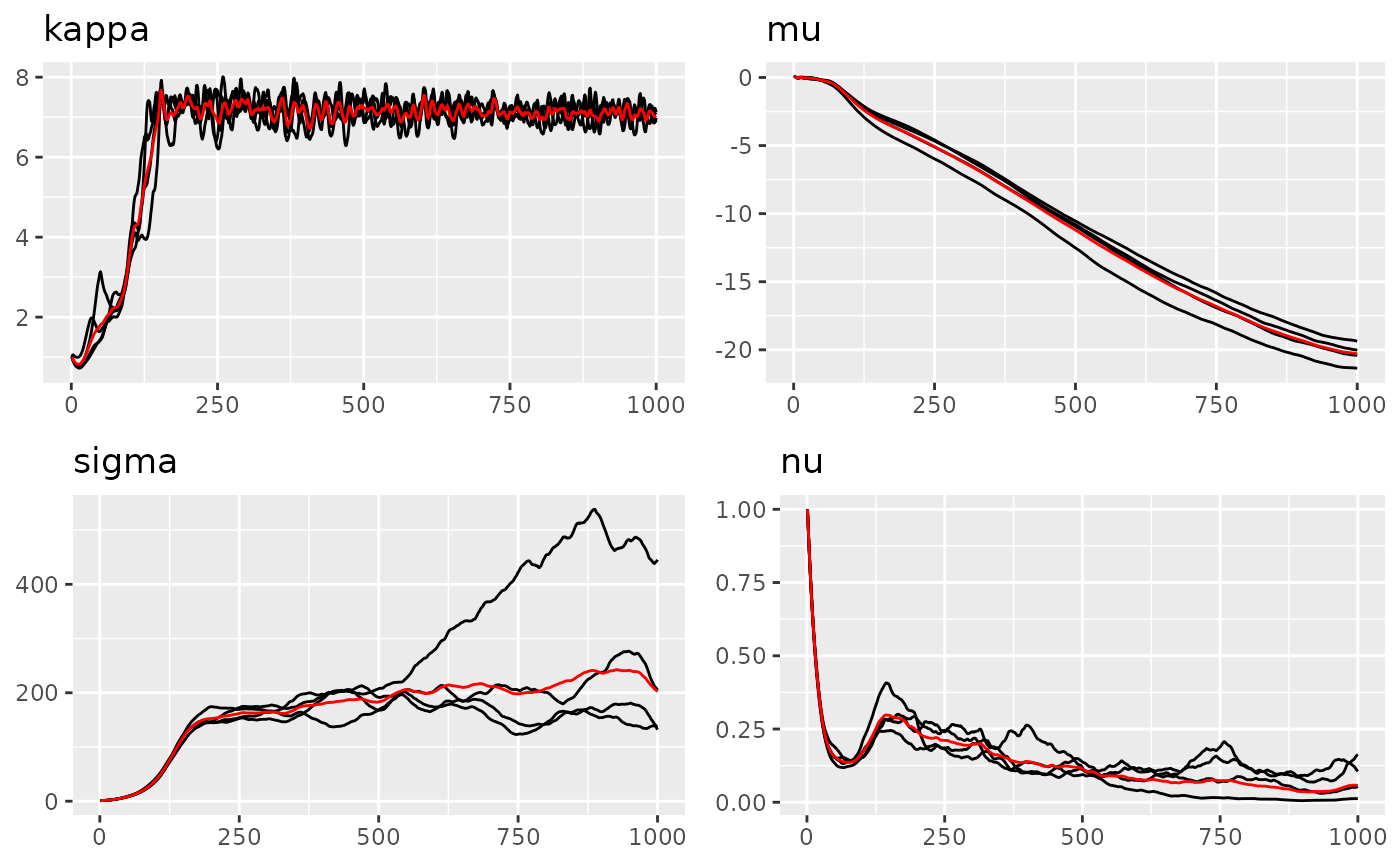
#> Last estimates:
#> $kappa
#> [1] 6.086098
#>
#> $mu
#> [1] -11.24909
#>
#> $sigma
#> [1] 35.61247
#>
#> $nu
#> [1] 0.6562881
traceplot(fit_nig, hline = c(0.1, 2))
#> Last estimates:
#> $sigma
#> [1] 0.09821712
Kringing
Kringing is a method for predicting the value of a random field at an unobserved location based on observations of the field at other locations.
We can use predict function in ngme2 to do
kringing.
# create new observations
locs <- graph$get_mesh_locations()
X <- as.data.frame(locs)
names(X) <- c("edge_number", "distance_on_edge")

preds <- predict(
  fit_nig,
  data = X,
  map = list(graph = locs)
)

# plot the prediction
graph$plot_function(preds$mean)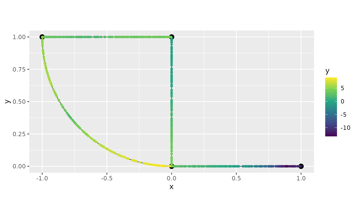
# compare with the true data
graph$plot(data = "y")