Combined Gaussian and NIG Noise Models

library(ngme2)
#> This is ngme2 of version 0.7.0
#> - See our homepage: https://davidbolin.github.io/ngme2 for more details.
set.seed(123) # For reproducibility

Introduction

This vignette introduces a special feature of the ngme2 package: the ability to model latent processes driven by a combination of both Gaussian and Normal Inverse Gaussian (NIG) noise. This mixed noise model provides greater flexibility in capturing complex distributional patterns in your data that may exhibit both heavy tails and Gaussian components.

Background: Understanding Mixed Noise Models

In many real-world applications, the observed data may result from processes affected by multiple sources of randomness with different distributional characteristics. The normal_nig noise model in ngme2 provides a powerful way to account for this by combining:

Normal (Gaussian) noise: Symmetric, light-tailed noise following a normal distribution.
Normal Inverse Gaussian (NIG) noise: A flexible, heavy-tailed distribution that can capture skewness and excess kurtosis.

The NIG distribution is a flexible four-parameter continuous probability distribution that can handle asymmetry and heavy tails. By combining it with normal noise, we can model complex stochastic behaviors more accurately.

Mathematical Formulation

The combined Normal-NIG noise model can be represented as:

$\epsilon_t = \epsilon_t^{NIG} + \epsilon_t^{Normal}$

where:

$\epsilon_t^{NIG}$ follows an NIG distribution with parameters $\mu$ , $\sigma_{NIG}$ , and $\nu$
$\epsilon_t^{Normal}$ follows a normal distribution with standard deviation $\sigma_{Normal}$

The NIG component itself is often constructed as:

$\epsilon_t^{NIG} = \delta + \mu V_t + \sigma_{NIG} \sqrt{V_t} Z_t$

where: - $\delta = -\mu$ (for identifiability) - $V_t$ follows an inverse Gaussian distribution with parameters related to $\nu$ - $Z_t$ is standard normal

Simulating Data with Mixed Normal-NIG Noise

Let’s simulate a dataset that exhibits both Gaussian and NIG noise components. We’ll create an AR(1) process driven by this mixed noise:

# Set parameters
n_obs <- 1000
sigma_eps <- 0.5  # Measurement noise (observation error)
alpha <- 0.5      # AR(1) coefficient
mu <- 2           # NIG parameter mu
delta <- -mu      # NIG parameter delta (typically set to -mu)
sigma_nig <- 3    # NIG noise scale
nu <- 1           # NIG shape parameter
sigma_normal <- 2  # Normal noise standard deviation

# First we generate V. V_i follows inverse Gaussian distribution
trueV <- ngme2::rig(n_obs, nu, nu, seed = 10)

# Generate the NIG noise component
nig_noise <- delta + mu*trueV + sigma_nig * sqrt(trueV) * rnorm(n_obs)

# Add normal noise component
mixed_noise <- nig_noise + rnorm(n_obs, mean=0, sd=sigma_normal)

# Generate the AR(1) process
trueW <- Reduce(function(x,y){y + alpha*x}, mixed_noise, accumulate = TRUE)

# Add measurement noise to get observations
Y <- trueW + rnorm(n_obs, mean=0, sd=sigma_eps)

# Add some fixed effects
x1 <- runif(n_obs)
x2 <- rexp(n_obs)
beta <- c(-3, -1, 2)
X <- model.matrix(~x1 + x2)  # design matrix
Y <- as.numeric(Y + X %*% beta)

# Plot the simulated data
par(mfrow=c(2,1), mar=c(4,4,2,1))
plot(Y, type="l", main="Simulated observations with Normal-NIG noise", 
     xlab="Time", ylab="Value")
plot(mixed_noise, type="l", main="Underlying Normal-NIG noise", 
     xlab="Time", ylab="Value")

Fitting Models with Normal-NIG Noise

The ngme2 package provides the noise_normal_nig() function to specify a combined Normal-NIG noise model. Let’s fit our simulated data:

# Fit model with Normal-NIG noise
ngme_out <- ngme(
  Y ~ x1 + x2 + f(
    1:n_obs,
    name = "my_ar",
    model = "ar1",
    # noise = noise_normal_nig()  # This specifies the combined noise model
    noise = list(noise_nig(mu=2, sigma_nig=3, nu=1), noise_normal(sigma_normal=1))
  ),
  data = data.frame(x1=x1, x2=x2, Y=Y),
  control_opt = control_opt(
    burnin = 100,
    iterations = 5000,
    std_lim = 0.4,
    n_parallel_chain = 4,
    seed = 3
  )
)
#> Starting estimation... 
#> 
#> Starting posterior sampling... 
#> Posterior sampling done! 
#> Note:
#>       1. Use ngme_post_samples(..) to access the posterior samples.
#>       2. Use ngme_result(..) to access different latent models.

# Show model summary
summary(ngme_out)
#> *** Ngme object ***
#> 
#> Fixed effects: 
#> (Intercept)          x1          x2 
#>       -2.62       -1.50        1.91 
#> 
#> Models: 
#> $my_ar
#>   Model type: AR(1)
#>       rho = 0.479
#>   Noise type: NORMAL_NIG
#>   Noise parameters: 
#>       mu = 2.15
#>       sigma_nig = 3.46
#>       nu = 1.73
#>       sigma_normal = 0.916
#> 
#> Measurement noise: 
#>   Noise type: NORMAL
#>   Noise parameters: 
#>       sigma = 0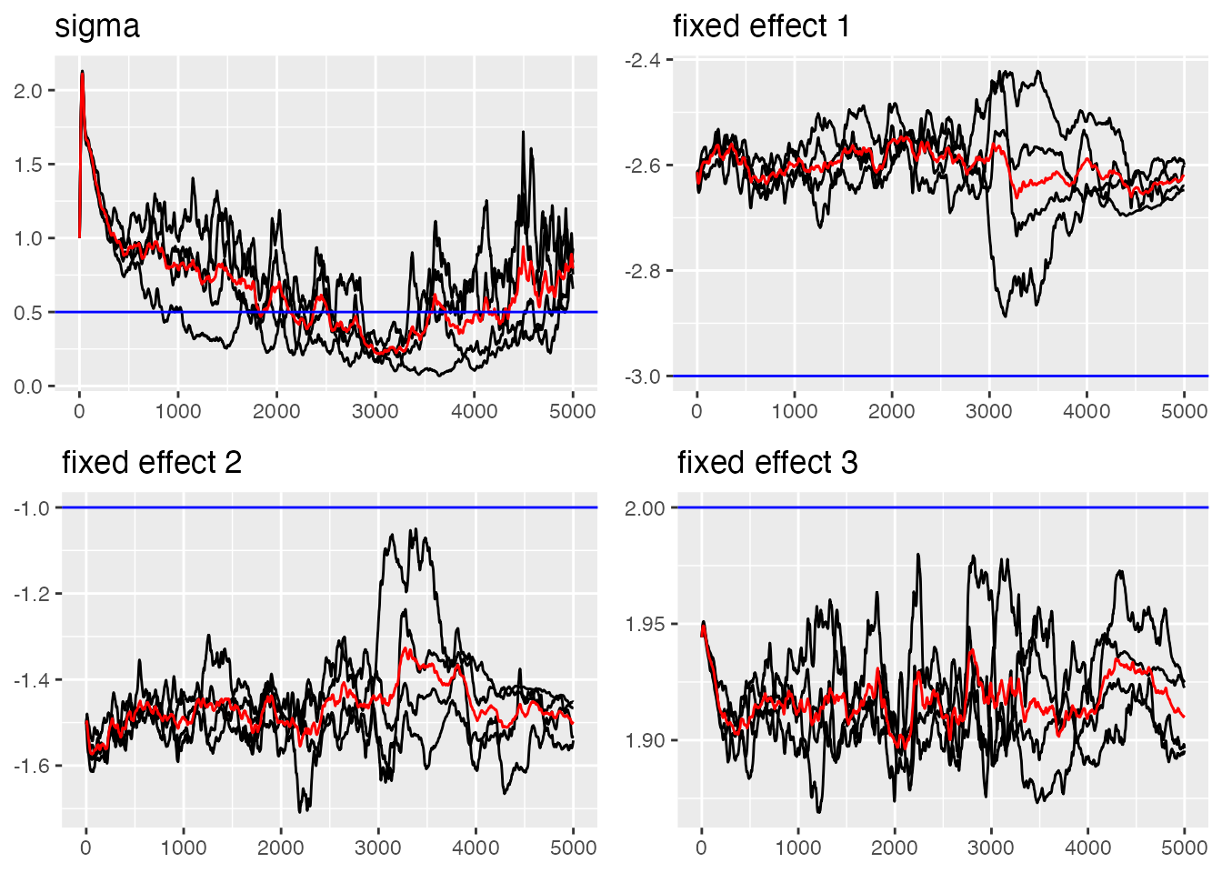.781
#> 
#> 
#> Number of replicates is  1

traceplot(ngme_out, hline = c(sigma_eps, beta))

#> Last estimates:
#> $sigma
#> [1] 0.7936722
#> 
#> $`fixed effect 1`
#> [1] -2.621681
#> 
#> $`fixed effect 2`
#> [1] -1.497698
#> 
#> $`fixed effect 3`
#> [1] 1.909849
traceplot(ngme_out, "my_ar", hline=c(alpha, mu, sigma_nig, sigma_normal, nu))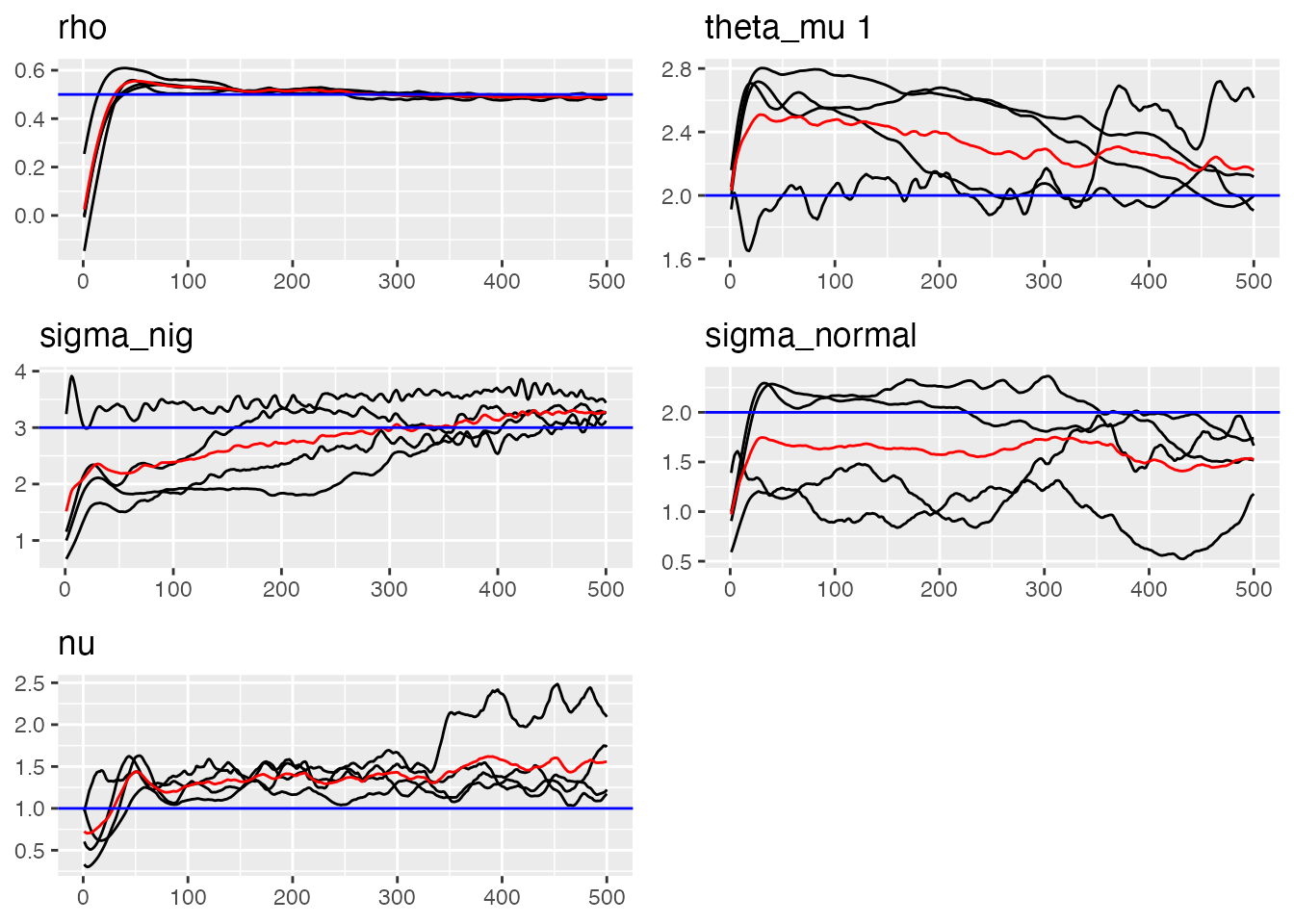

#> Last estimates:
#> $rho
#> [1] 0.476164
#> 
#> $`theta_mu 1`
#> [1] 2.163596
#> 
#> $sigma_nig
#> [1] 3.4401
#> 
#> $sigma_normal
#> [1] 1.111303
#> 
#> $nu
#> [1] 1.736965

Visualizing the Results

We can use the traceplot() function to see the estimated parameters trajectories:

# Plot traces for fixed effects
traceplot(ngme_out, hline=c(sigma_eps, beta))

# Plot traces for AR(1) component
traceplot(ngme_out, "my_ar", hline=c(alpha, mu, sigma_nig, nu, sigma_normal))

Advanced Features of the Normal-NIG Noise

The noise_normal_nig() function provides several customization options:

# Specifying initial values for parameters
custom_noise <- noise_normal_nig(
  mu = 2,             # Initial value for mu
  sigma_nig = 3,      # Initial value for NIG sigma
  nu = 1,             # Initial value for nu
  sigma_normal = 0.8  # Initial value for normal sigma
)

Real-world Applications

The combined Normal-NIG noise model is particularly useful in:

Financial time series: Where data often exhibits both heavy tails (extreme events) and normal fluctuations
Environmental data: Such as pollution levels or climate measurements that may show a mixture of different random behaviors
Epidemiological studies: Disease spread can follow patterns with both regular fluctuations and occasional outbreaks
Spatial statistics: When combining both smooth variations and occasional sharp discontinuities

Conclusion

The noise_normal_nig() function in ngme2 provides a powerful way to model complex random processes that exhibit both heavy-tailed and normal characteristics. By combining Normal and NIG noise components, you can create more flexible and realistic models for your data.

When your data shows signs of both heavy tails and Gaussian components, consider using this mixed noise model rather than restricting yourself to a single noise distribution. The examples in this vignette demonstrate how to simulate, fit, and analyze such models, helping you make better use of the ngme2 package’s advanced features. ****

ngme2 Team

2025-05-22