Ngme2 - A Unified, Efficient, and Flexible non-Gaussian Modeling Framework • ngme2

Introduction

Latent Gaussian models (LGMs) have emerged as a cornerstone of modern statistical inference, providing a powerful framework for modeling hierarchical dependencies in data.

Despite their versatility, LGMs encounter fundamental limitations when applied to data exhibiting non-Gaussian characteristics. The Gaussian assumption imposes inherent constraints that may be overly restrictive for many real-world phenomena. Some common non-Gaussian features exhibited by real world data include asymmetry, heavy tails, and non-smoothness.

ngme2 R package is a unified, efficient, and flexible modeling software for modeling non-Gaussian data. It is the updated version of ngme, which was first introduced in (Asar et al. 2020)

Features

Support temporal models like AR(1), Ornstein−Uhlenbeck and random walk processes, and spatial models like Matern fields.
Support latent processes driven by non-Gaussian noises (normal inverse Gaussian(NIG), generalized asymmetric Laplace (GAL), etc).
Support non-Gaussian, and correlated measurement noises.
Support kriging prediction at unknown locations.
Support latent processes and random-effects model for longitudinal data.
Support the bivariate type-G model, which can model 2 non-Gaussian fields jointly (Bolin and Wallin 2019).
Support the separable space-time model, and non-separable space-time model.
Support the user-defined model via generic and generic_ns functions.
Provide estimation diagnostics, and cross-validation for model selection.

Model Framework

The package Ngme2 implements the latent linear non-Gaussian model (LLnGM) framework, which uses flexible operator formulations to describe data, latent processes, and noise in a unified way:

$\begin{align} \text{Data:} \quad & \mathbf{Y} = \mathbf{A}\mathbf{W} + \mathbf{X}\boldsymbol{\beta} + \boldsymbol{\epsilon}^{(1)} \tag{eq:data}\\ \text{Process:} \quad & \mathbf{K}(\boldsymbol{\theta})\mathbf{W} = \boldsymbol{\epsilon}^{(2)} \tag{eq:process}\\ \text{Noise:} \quad & \boldsymbol{\epsilon}^{(i)} | \mathbf{V}^{(i)} \sim \mathcal{N}(\mathbf{m}^{(i)}, \boldsymbol{\Sigma}^{(i)}), \quad i = 1, 2 \tag{eq:noise} \\ & \mathbf{m}^{(i)} = \boldsymbol{\mu}^{(i)}({\boldsymbol{\theta}}) \odot \left( \mathbf{V}^{(i)} - \mathbf{h}^{(i)} \right), \\ & \boldsymbol{\Sigma}^{(i)} = \text{diag}(\boldsymbol{\sigma}^{(i)}({\boldsymbol{\theta}}) \odot \boldsymbol{\sigma}^{(i)}({\boldsymbol{\theta}}) \odot \mathbf{V}^{(i)}) \\ \text{Distribution:} \quad & \mathbf{V}_j^{(i)} \overset{\text{iid}}{\sim} \text{GIG}(\mathbf{p}_j^{(i)}(\boldsymbol{\theta}), \mathbf{a}_j^{(i)}(\boldsymbol{\theta}), \mathbf{b}_j^{(i)}(\boldsymbol{\theta})) \tag{eq:distribution} \quad i = 1, 2, \quad j = 1, \ldots, n_i \end{align}$

The data model links observations $\mathbf{Y} \in \mathbb{R}^{n_1}$ to the latent process $\mathbf{W} \in \mathbb{R}^{n_2}$ through the observation matrix $\mathbf{A} \in \mathbb{R}^{n_1 \times n_2}$ , adds fixed effects $\mathbf{X}\boldsymbol{\beta}$ , and allows non-Gaussian measurement noise $\boldsymbol{\epsilon}^{(1)} \in \mathbb{R}^{n_1}$ .

The process model specifies the core dependency structure of $\mathbf{W}$ via the operator matrix $\mathbf{K}(\boldsymbol{\theta}) \in \mathbb{R}^{n_2 \times n_2}$ , which is driven by potentially non-Gaussian noise $\boldsymbol{\epsilon}^{(2)} \in \mathbb{R}^{n_2}$ . This operator-based formulation unifies a wide spectrum of model structures, from simple random effects to complex spatio-temporal patterns.

Here $\odot$ denotes element-wise multiplication. The noise model defines $\boldsymbol{\epsilon}^{(1)}$ and $\boldsymbol{\epsilon}^{(2)}$ through normal mean-variance mixtures conditioned on the GIG mixing vectors $\mathbf{V}^{(1)} \in \mathbb{R}^{n_1}$ and $\mathbf{V}^{(2)} \in \mathbb{R}^{n_2}$ . The parameter vector $\boldsymbol{\theta}$ collects all model parameters.

Here is a simple template for using the core function ngme to model the single response:

ngme(
  formula=Y ~ x1 + x2 + f(index, model=ar1(mesh_1d), noise=noise_nig()),
  data=data.frame(Y=Y, x1=x1, x2=x2, index=index),
  family = "normal"
)

Here, function f is for modeling the stochastic process W with Gaussian or non-Gaussian noise, we will discuss this later. noise stands for the measurement noise distribution. In this case, the model will have a Gaussian likelihood.

Non-Gaussian Model

Here we assume the non-Gaussian process is a type-G Lévy process, whose increments can be represented as location-scale mixtures: $\gamma + \mu V + \sigma \sqrt{V}Z,$ where $\gamma, \mu, \sigma$ are parameters, $Z\sim N(0,1)$ is independent of $V$ , and $V$ is a positive infinitely divisible random variable. This results in the following form, where $K$ is the operator part:

$KW|V \sim N(\gamma + \mu V, \sigma^2 \, \text{diag}(V)),$ where $\mu$ and $\sigma$ can be non-stationary.

One example in ngme2 is the normal inverse Gaussian (NIG) noise, where $V$ follows an Inverse Gaussian distribution with parameter $\nu$ (IG( $\nu$ , $\nu$ )).

A random variable $V$ follows an inverse Gaussian distribution with parameters $\eta_1$ and $\eta_2$ , denoted by $V\sim \text{IG}(\eta_1,\eta_2)$ , if it has probability density function (pdf) given by $\pi(v) = \frac{\sqrt{\eta_2}}{\sqrt{2\pi v^3}} \exp\left\{-\frac{\eta_1}{2}v - \frac{\eta_2}{2v} + \sqrt{\eta_1\eta_2}\right\},\quad \eta_1,\eta_2>0.$ We can generate samples from an inverse Gaussian distribution with parameters $\eta_1$ and $\eta_2$ by generating samples from the generalized inverse Gaussian distribution with parameters $p=-1/2$ , $a=\eta_1$ and $b=\eta_2$ . The rGIG function can be used to generate samples from the generalized inverse Gaussian distribution.

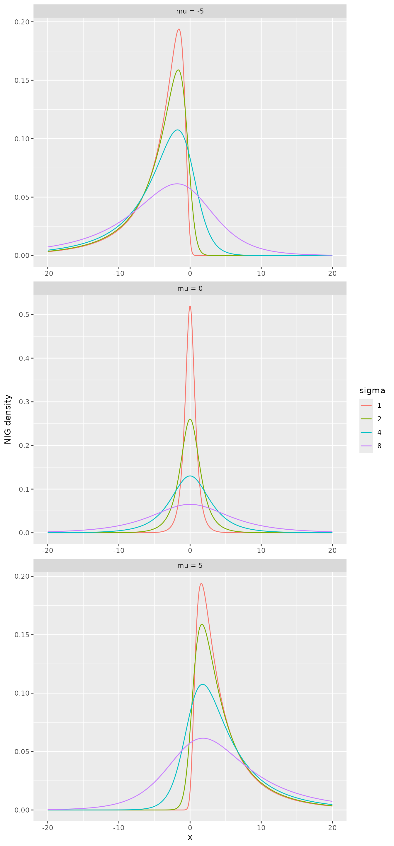
If $V\sim \text{IG}(\eta_1,\eta_2)$ , and $X = \gamma +\mu V + \sigma \sqrt{V}Z$ , with $Z\sim N(0,1)$ independent of $V$ , then $X$ follows a normal inverse Gaussian (NIG) distribution with pdf $\pi(x) = \frac{e^{\sqrt{\eta_1\eta_2}+\mu(x-\gamma)/\sigma^2}\sqrt{\eta_2\mu^2/\sigma^2+\eta_1\eta_2}}{\pi\sqrt{\eta_2\sigma^2+(x-\gamma)^2}} K_1\left(\sqrt{(\eta_2\sigma^2+(x-\gamma)^2)(\mu^2/\sigma^4+\eta_1/\sigma^2)}\right),$ where $K_1$ is a modified Bessel function of the third kind. In this form, the NIG density is overparameterized, so we set $\eta_1=\eta_2=\eta$ , which results in $E(V)=1$ . Thus, we have the parameters $\mu$ , $\gamma$ , and $\eta$ .

The NIG model assumes that the stochastic variance $V_i$ follows an inverse Gaussian distribution with parameters $\eta$ and $\eta h_i^2$ , where $h_i = \int_{\mathcal{D}} \varphi_i(\mathbf{s}) d\mathbf{s}.$

The following figure shows the density of NIG distribution with different parameters.

Parameter Estimation

Ngme2 does maximum likelihood estimation through preconditioned stochastic gradient descent. See Model estimation and prediction for more details.
Multiple chains are supported for better convergence checks.
Different stochastic optimization algorithms can be used for the optimization process. See ?ngme_optimizers for more details.
Different convergence checks are supported.

Ngme Model Structure

Specify the driven noise

There are 2 types of common noise involved in the model, one is the innovation noise of a stochastic process, one is the measurement noise of the observations. They can be both specified by noise_<type> function.

For now we support normal, skew_t, NIG, and GAL noises.

The R class ngme_noise has the following interface:

library(fmesher)
library(splancs)
library(lattice)
library(ggplot2)
library(grid)
library(gridExtra)
library(viridis)
library(ngme2)

noise_normal(sigma = 1) # normal noise
#> Noise type: NORMAL
#> Noise parameters: 
#>     sigma = 1
noise_nig(mu = 1, sigma = 2, nu = 1) # nig noise
#> Noise type: NIG
#> Noise parameters: 
#>     mu = 1
#>     sigma = 2
#>     nu = 1
noise_nig( # non-stationary nig noise
  B_mu = matrix(c(1:10), ncol = 2),
  theta_mu = c(1, 2),
  B_sigma = matrix(c(1:10), ncol = 2),
  theta_sigma = c(1, 2),
  nu = 1
)
#> Noise type: NIG
#> Noise parameters: 
#>     theta_mu = 1, 2
#>     theta_sigma = 1, 2
#>     nu = 1
noise_skew_t(mu = 1, sigma = 2, nu = 1) # skew_t noise
#> Noise type: SKEW_T
#> Noise parameters: 
#>     mu = 1
#>     sigma = 2
#>     nu = 1

Notice that the 3rd example is defined for non-stationary NIG noise. In general, we can define non-stationary noise by the following: where $\mu = \mathbf{B}_{\mu} \mathbf{\theta}_{\mu}$ , $\sigma = \exp(\mathbf{B}_{\sigma} \mathbf{\theta}_{\sigma})$ , and $\nu = \exp(\mathbf{B}_{\nu} \mathbf{\theta}_{\nu})$

ngme_noise(
  type,           # the type of noise
  theta_mu,       # mu parameter
  theta_sigma,    # sigma parameter
  theta_nu,       # nu parameter
  B_mu,           # basis matrix for non-stationary mu
  B_sigma,        # basis matrix for non-stationary sigma
  B_nu            # basis matrix for non-stationary nu
)

It will construct the following noise structure:

$- \mathbf{\mu} + \mathbf{\mu} V + \mathbf{\sigma} \sqrt{V} Z$

Additionally, ngme2 provides a special combined noise model that merges both Gaussian and NIG noise components:

noise_normal_nig(
  mu = 2, # NIG parameter mu
  sigma_nig = 3, # NIG noise scale
  nu = 1, # NIG shape parameter
  sigma_normal = 0.8 # Normal noise standard deviation
)
#> Noise type: NORMAL_NIG
#> Noise parameters: 
#>     mu = 2
#>     sigma_nig = 3
#>     nu = 1
#>     sigma_normal = 0.8

This combined noise model is particularly useful for complex processes where both normal variations and heavy-tailed events occur. For more details, see the dedicated vignette: vignette("normal-nig-noise", package = "ngme2").

Specify stochastic process with `f` function

The middle layer is the stochastic process, in R interface, it is represented as a f function. The process can be specified by different noise structure. See ?ngme_model_types() for more details.

Some examples of using f function to specify ngme_model:

f(1:10, model = ar1(), noise = noise_nig())
#> Model type: AR(1)
#>     rho = 0
#> Noise type: NIG
#> Noise parameters: 
#>     mu = 0
#>     sigma = 1
#>     nu = 1

One useful model would be the SPDE model with Gaussian or non-Gaussian noise, see the vignette for details.

Specifying latent models with formula in `ngme`

The latent model can be specified additively as a formula argument in ngme function together with fixed effects.

We use R formula to specify the latent model. We can specify the model using f within the formula.

For example, the following formula

formula <- Y ~ x1 + f(
  x2,
  model = ar1(),
  noise = noise_nig()
) + f(x3,
  model = rw1(),
  noise = noise_normal()
)

corresponds to the model

$Y = \beta_0 + \beta_1 x_1 + W_1(x_2) + W_2(x_3) + \epsilon,$ where $W_1$ is an AR(1) process, $W_2$ is a random walk 1 process. $x_2$ is random effects.. . By default, we have intercept. The distribution of the measurement error $\epsilon$ is given in the ngme function.

The entire model can be fitted, along with the specification of the distribution of the measurement error through the ngme function:

ngme(
  formula = formula,
  family = noise_normal(sigma = 0.5),
  data = data.frame(Y = 1:5, x1 = 2:6, x2 = 3:7, x3 = 4:8),
  control_opt = control_opt(
    estimation = FALSE
  )
)
#> *** Ngme object ***
#> 
#> Fixed effects: 
#> (Intercept)          x1 
#>       7.365      -0.869 
#> 
#> Models: 
#> $field1
#>   Model type: AR(1)
#>       rho = 0
#>   Noise type: NIG
#>   Noise parameters: 
#>       mu = 0
#>       sigma = 1
#>       nu = 1
#> 
#> $field2
#>   Model type: Random walk (order 1)
#>       No parameter.
#>   Noise type: NORMAL
#>   Noise parameters: 
#>       sigma = 1
#> 
#> Measurement noise: 
#>   Noise type: NORMAL
#>   Noise parameters: 
#>       sigma = 0.5

It gives the ngme object, which has three parts:

Fixed effects (intercept and x1)
Measurement noise (normal noise)
Latent models (contains 2 models, ar1 and rw1)

We can turn the estimation = TRUE to start estimating the model.

Convergence check methods

ngme2 can monitor convergence with three optional diagnostics. They all run at each checkpoint (every iters_per_check iterations, default iterations / n_batch). Checks only begin after n_min_batch checkpoints have accumulated.

Gelman–Rubin R̂ (R_hat_conv_check, max_R_hat)
Compares between- and within-chain variance for each parameter; pass if R_hat <= max_R_hat (default 1.1). Requires at least 2 chains (n_parallel_chain >= 2).
Trend/Std diagnostic (trend_std_conv_check)
Uses the last n_slope_check checkpoints (default 3). Passes when both hold for each parameter:
- sqrt(var) / |mean| <= std_lim (default 0.01)
- |linear slope over last n_slope_check means| <= trend_lim (default 0.01).
Pflug diagnostic (pflug_conv_check, pflug_alpha)
For each chain, checks pflug_sum < pflug_alpha * max_pflug_sum in the latest batch (default pflug_alpha = 1). If all chains satisfy this, convergence is declared regardless of the other two checks.

Combination rule: - A parameter is considered converged if any enabled diagnostic passes for it (R̂ or Trend/Std).
- Overall convergence is reached when all parameters are converged, or when the Pflug diagnostic passes for all chains.

Key control knobs (set via control_opt()):

ctrl <- control_opt(
  n_batch = 10,               # number of checkpoints
  n_min_batch = 3,            # don't check before this many checkpoints
  n_slope_check = 3,          # window for trend regression
  R_hat_conv_check = TRUE,
  max_R_hat = 1.1,
  trend_std_conv_check = TRUE,
  std_lim = 0.01,
  trend_lim = 0.01,
  pflug_conv_check = TRUE,
  pflug_alpha = 1,
  print_check_info = TRUE     # print per-check diagnostics
)

Recommendations: - Use at least two chains for R̂; with one chain only Trend/Std and Pflug can run. - If checks trigger too early, increase n_min_batch or loosen std_lim / trend_lim. - Pflug is inexpensive; keep it on unless it yields false positives in your model.

A simple example - AR1 process with nig noise

Now let’s see an example of an AR1 process with nig noise. The process is defined as

$W_i = \rho W_{i-1} + \epsilon_i,$ Here, $\epsilon_1, ..,\epsilon_n$ is the iid NIG noise. And, it is easy to verify that $K\mathbf{W} = \boldsymbol\epsilon$ , where $K = \begin{bmatrix} \sqrt{1-\rho^2} \\ -\rho & 1 \\ & \ddots & \ddots \\ & & -\rho & 1 \end{bmatrix}$

n_obs <- 500
sigma_eps <- 0.5
rho <- 0.5
mu <- 2
delta <- -mu
sigma <- 3
nu <- 1

# First we generate V. V_i follows inverse Gaussian distribution
trueV <- ngme2::rig(n_obs, nu, nu, seed = 10)

# Then generate the nig noise
mynoise <- delta + mu * trueV + sigma * sqrt(trueV) * rnorm(n_obs)
trueW <- Reduce(function(x, y) {
  y + rho * x
}, mynoise, accumulate = T)
Y <- trueW + rnorm(n_obs, mean = 0, sd = sigma_eps)

# Add some fixed effects
x1 <- runif(n_obs)
x2 <- rexp(n_obs)
beta <- c(-3, -1, 2)
X <- (model.matrix(Y ~ x1 + x2)) # design matrix
Y <- as.numeric(Y + X %*% beta)

Now let’s fit the model using ngme. Here we can use control_opt to modify the control variables for the ngme. See ?control_opt for more optioins.

# Fit the model with the AR1 model
fit_nig <- ngme(
  Y ~ x1 + x2 + f(
    1:n_obs,
    name = "my_ar",
    model = ar1(),
    noise = noise_nig()
  ),
  data = data.frame(x1 = x1, x2 = x2, Y = Y),
  control_opt = control_opt(
    burnin = 100,
    iterations = 2000,
    n_parallel_chain = 4,
    seed = 3,
    pflug_conv_check = TRUE,
    pflug_alpha = 1
  )
)
#> Starting estimation... 
#> 
#> Starting posterior sampling... 
#> Posterior sampling done! 
#> Average standard deviation of the posterior W:  4.325882 
#> Note:
#>       1. Use ngme_post_samples(..) to access the posterior samples.
#>       2. Use ngme_result(..) to access different latent models.

Next we can read the result directly from the object.

fit_nig
#> *** Ngme object ***
#> 
#> Fixed effects: 
#> (Intercept)          x1          x2 
#>       -2.91       -1.38        2.02 
#> 
#> Models: 
#> $my_ar
#>   Model type: AR(1)
#>       rho = 0.568
#>   Noise type: NIG
#>   Noise parameters: 
#>       mu = 1.87
#>       sigma = 2.96
#>       nu = 0.899
#> 
#> Measurement noise: 
#>   Noise type: NORMAL
#>   Noise parameters: 
#>       sigma = 0.583

The estimation results are close to the real parameter.

We can also use the traceplot function to see the estimation traceplot.

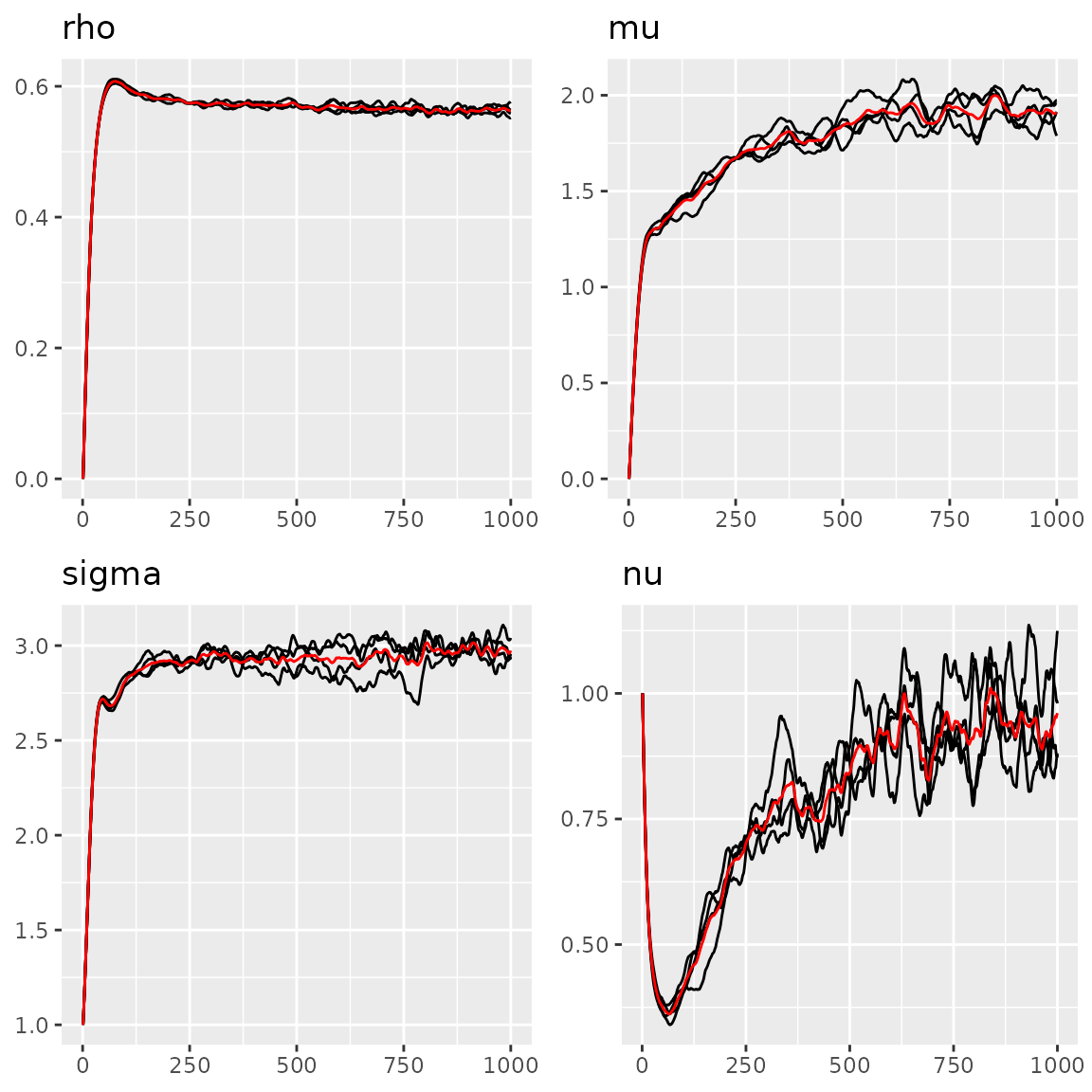
traceplot(fit_nig, "my_ar", hline = c(rho, mu, sigma, nu))

Parameters of the AR1 model

#> Last estimates:
#> $rho
#> [1] 0.5678771
#> 
#> $mu
#> [1] 1.857891
#> 
#> $sigma
#> [1] 2.995272
#> 
#> $nu
#> [1] 0.9055304

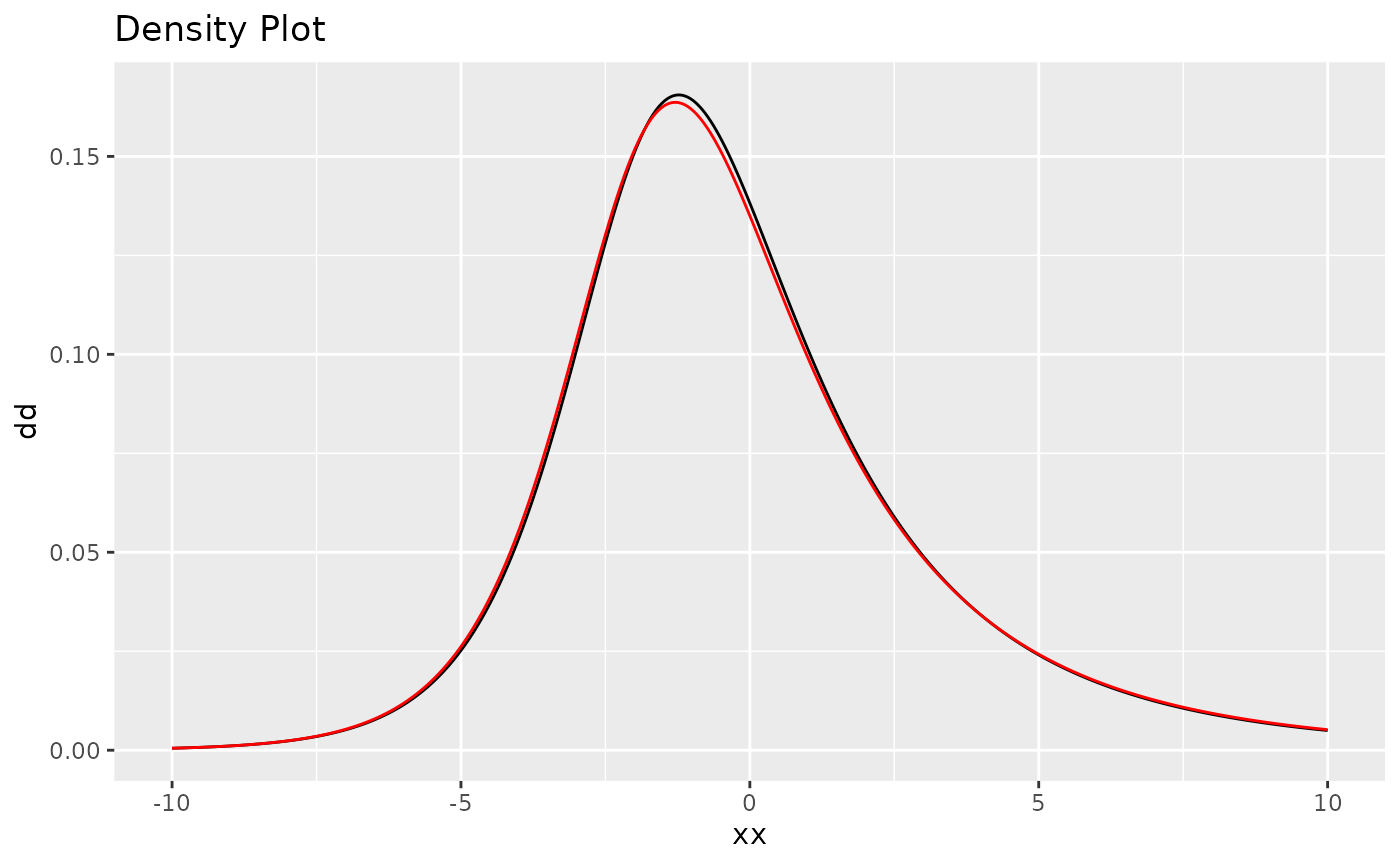
We can also do a density comparison with the estimated noise and the true NIG noise, we can see they are very close:

# fit_nig$replicates[[1]] means for the 1st replicate
plot(
  fit_nig$replicates[[1]]$models[[1]]$noise,
  noise_nig(mu = mu, sigma = sigma, nu = nu)
)

Paraná dataset

The rainfall data from Paraná (Brazil) is collected by the National Water Agency in Brazil (Agencia Nacional de Águas, ANA, in Portuguese). ANA collects data from many locations over Brazil, and all these data are freely available from the ANA website (http://www3.ana.gov.br/portal/ANA).

We will briefly illustrate the command we use, and the result of the estimation.

library(INLA)
#> Loading required package: Matrix
#> This is INLA_25.04.16 built 2025-04-16 08:17:54 UTC.
#>  - See www.r-inla.org/contact-us for how to get help.
#>  - List available models/likelihoods/etc with inla.list.models()
#>  - Use inla.doc(<NAME>) to access documentation
#>  - Consider upgrading R-INLA to testing[25.12.02] or stable[25.10.19] (require R-4.5)
#> 
#> Attaching package: 'INLA'
#> The following object is masked from 'package:ngme2':
#> 
#>     f
data(PRprec)
data(PRborder)

# Create mesh
coords <- as.matrix(PRprec[, 1:2])
prdomain <- fmesher::fm_nonconvex_hull(coords, -0.03, -0.05, resolution = c(100, 100))
prmesh <- fmesher::fm_mesh_2d(boundary = prdomain, max.edge = c(0.45, 1), cutoff = 0.2)

# monthly mean at each location
Y <- rowMeans(PRprec[, 12 + 1:31]) # 2 + Octobor

ind <- !is.na(Y) # non-NA index
Y <- Y_mean <- Y[ind]
coords <- as.matrix(PRprec[ind, 1:2])
seaDist <- apply(spDists(coords, PRborder[1034:1078, ],
  longlat = TRUE
), 1, min)

Plot the data:

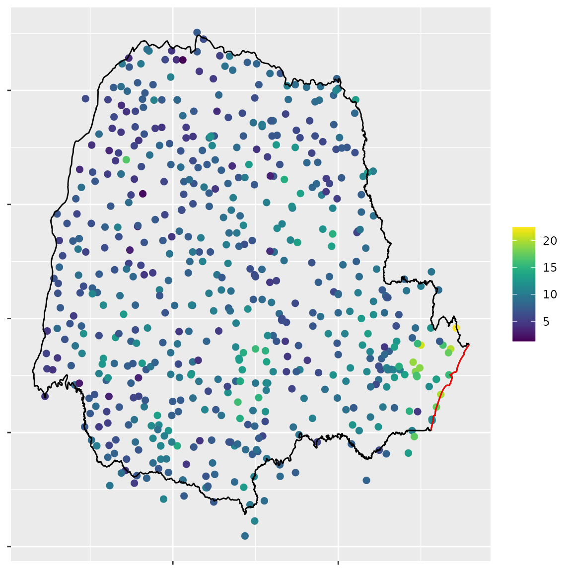
Mean of the rainfall in Octobor 2012 in Paraná

# Define the control options
control <- control_opt(
  iterations = 2000,
  n_min_batch = 4,
  n_batch = 10,
  n_parallel_chain = 4,
  optimizer = precond_sgd(),
  print_check_info = FALSE,
  seed = 16
)

parana_fit <- ngme(
  formula = Y ~ 1 +
    f(coords,
      model = matern(
        mesh = prmesh,
      ),
      noise = noise_nig(),
      name = "spde"
    ),
  data = data.frame(Y = Y),
  family = "normal",
  control_opt = control
)
#> Starting estimation... 
#> 
#> Starting posterior sampling... 
#> Posterior sampling done! 
#> Average standard deviation of the posterior W:  2.87084 
#> Note:
#>       1. Use ngme_post_samples(..) to access the posterior samples.
#>       2. Use ngme_result(..) to access different latent models.

# traceplots
## fixed effects and measurement error
traceplot(parana_fit)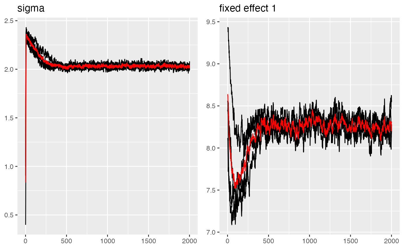

#> Last estimates:
#> $sigma
#> [1] 2.042884
#> 
#> $`fixed effect 1`
#> [1] 8.297917

## spde model
traceplot(parana_fit, "spde")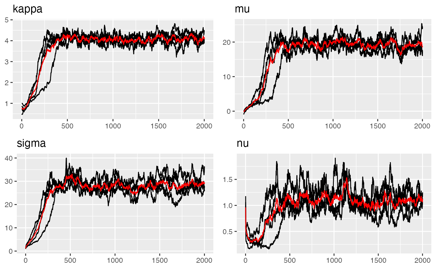

#> Last estimates:
#> $kappa
#> [1] 4.124553
#> 
#> $mu
#> [1] 18.75537
#> 
#> $sigma
#> [1] 29.15408
#> 
#> $nu
#> [1] 1.122146

Parameter estimation results:

#> $fixed_effects
#> (Intercept) 
#>    8.241518 
#> 
#> $sigma
#> [1] 2.027681
#> $kappa
#> [1] 4.100826
#> 
#> $mu
#> [1] 19.20593
#> 
#> $sigma
#> [1] 28.8247
#> 
#> $nu
#> [1] 1.084761

Prediction

Now we can use the fitted model to do prediction by generating the prediction grid and giving the predict location.

nxy <- c(150, 100)
projgrid <- rSPDE::rspde.mesh.projector(prmesh,
  xlim = range(PRborder[, 1]),
  ylim = range(PRborder[, 2]), dims = nxy
)

xy.in <- inout(projgrid$lattice$loc, cbind(PRborder[, 1], PRborder[, 2]))

coord.prd <- projgrid$lattice$loc[xy.in, ]
plot(coord.prd, type = "p", cex = 0.1)
lines(PRborder)
points(coords[, 1], coords[, 2], pch = 19, cex = 0.5, col = "red")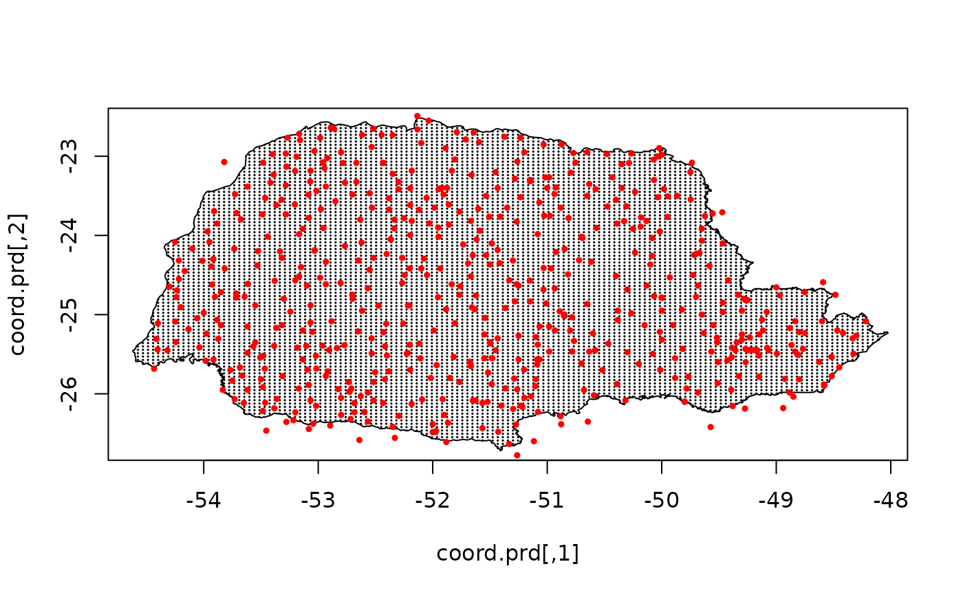


# Doing prediction by giving the predict location
pds <- predict(parana_fit, map = list(spde = coord.prd))
lp <- pds$mean
ggplot() +
  geom_point(aes(
    x = coord.prd[, 1], y = coord.prd[, 2],
    colour = lp
  ), size = 2, alpha = 1) +
  geom_point(aes(
    x = coords[, 1], y = coords[, 2],
    colour = Y_mean
  ), size = 2, alpha = 1) +
  scale_color_gradientn(colours = viridis(100)) +
  geom_path(aes(x = PRborder[, 1], y = PRborder[, 2])) +
  geom_path(aes(x = PRborder[1034:1078, 1], y = PRborder[
    1034:1078,
    2
  ]), colour = "red")

Model comparison with latent Gaussian model via cross-validation

We can also fit a latent Gaussian model and compare it with the NIG model via cross-validation. The following code shows how to do it. For the details of the cross-validation, see the cross-validation vignette.

parana_fit_gauss <- ngme(
  formula = Y ~ 1 +
    f(coords,
      model = matern(
        mesh = prmesh,
      ),
      noise = noise_normal(),
      name = "spde"
    ),
  data = data.frame(Y = Y),
  family = "normal",
  control_opt = control
)
#> Starting estimation... 
#> 
#> Starting posterior sampling... 
#> Posterior sampling done! 
#> Average standard deviation of the posterior W:  2.572308 
#> Note:
#>       1. Use ngme_post_samples(..) to access the posterior samples.
#>       2. Use ngme_result(..) to access different latent models.

cv <- cross_validation(
  list(
    gauss = parana_fit_gauss,
    nig = parana_fit
  ),
  type = "k-fold",
  seed = 13,
  n_gibbs_samples = 2000,
  n_burnin = 100,
  k = 10,
  print = FALSE
)
cv
#> $mean.scores
#>            MAE      MSE neg.CRPS neg.sCRPS
#> gauss 1.740767 5.230700 1.247329  1.457489
#> nig   1.730342 5.209617 1.244528  1.453643
#> 
#> $sd.scores
#>               MAE        MSE    neg.CRPS   neg.sCRPS
#> gauss 0.002581289 0.01328677 0.003350892 0.001549784
#> nig   0.003524973 0.02285076 0.003478937 0.001643864

As we can see, the NIG model has a slightly better cross-validation performance in most metrics.

References

Asar, Özgür, David Bolin, Peter J. Diggle, and Jonas Wallin. 2020. “Linear Mixed Effects Models for Non-Gaussian Continuous Repeated Measurement Data.” Journal of the Royal Statistical Society Series C: Applied Statistics 69 (5): 1015–65. https://doi.org/10.1111/rssc.12405.

Bolin, David, and Jonas Wallin. 2019. “Multivariate Type G Matérn Stochastic Partial Differential Equation Random Fields.” Journal of the Royal Statistical Society Series B: Statistical Methodology. https://doi.org/10.1111/rssb.12351.

Ngme2 - A Unified, Efficient, and Flexible non-Gaussian Modeling Framework

2025-12-10