Spatio-temporal models
David Bolin and Alexandre B. Simas
Created: 2024-10-23. Last modified: 2026-04-08.
Source:vignettes/spacetime.Rmd
spacetime.RmdIntroduction
The rSPDE package implements the following
spatio-temporal model
where
is a temporal interval and
is a spatial domain which can be an interval, a bounded subset of
or a metric graph. Here
is a spatial range parameter,
is a drift parameter which is in
for spatial domains that are intervals or metric graphs, and in
for spatial domains which are bounded subsets of
.
Further,
is a
-Wiener
process with spatial covariance operator
,
where
is a variance parameter. Thus, the model has two smoothness parameters
and
which are assumed to be integers. The model is therefore a
generalization of the spatio-temporal models introduced in Lindgren et al. (2024), where the
generalization is to allow for drift and to allow for metric graphs as
spatial domains. The model is implemented using a finite element
discretization of the corresponding precision operator
in both space and time, similarly to
the discretization introduced in Lindgren et al. (2024). This
parameterization of the drift term, using
in place of the standard
,
is chosen to simplify the enforcement of theoretical bounds on the range
of
,
ensuring that the equation remains well-posed and also providing
numerical stability for finite-dimensional approximations.
Implementation details
Let us begin by loading some packages needed for making the plots
The function spacetime.operators() can be used to define
the model. The function requires specifying the two smoothness
parameters, and the discretization points for the spatial and temporal
discretizations. The spatial discretization can be specified through a
mesh object from the fmesher package, as a graph from the
MetricGraph package, or as the mesh nodes for models on
intervals. The temporal discretization can be specified either by
specifying the mesh nodes or by providing a mesh object.
Assume that we want to define a model on the spatial interval and the temporal domain . We can then simply specify the mesh nodes as
s <- s_1d <- seq(from = 0, to = 20, length.out = 101)
t <- t_1d <- seq(from = 0, to = 10, length.out = 21)
We can now use spacetime.operators() to construct the
model
kappa <- 5
sigma <- 10
gamma <- 0.1
rho_1d <- 1
alpha <- 1
beta <- 1

op <- spacetime.operators(
  space_loc = s, time_loc = t,
  kappa = kappa, sigma = sigma, alpha = alpha,
  beta = beta, rho = rho_1d, gamma = gamma
)
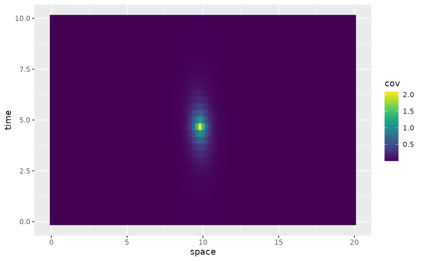
The spacetime.operators object has a
plot_covariances method which for univariate spatial
domains simply plots the covariance
for a fixed spatio-temporal location
specified by the indices in the spatial and temporal discretizations.
For example:
op$plot_covariances(t.ind = 15, s.ind = 50)
 The object
 op contains the matrices needed for evaluating
the model, and we have here initialized it by providing values for all
parameters.
We can simulate from the model using simulate():
u <- simulate(op)There is also built-in support for kriging prediction. To illustrate this, we use the simulation to create some noisy observations of the process. For this, we first construct the observation matrix linking the FEM basis functions to the locations where we want to simulate. We first randomly generate some observation locations and then construct the matrix.
n.obs <- 500

obs.loc <- data.frame(x = max(s) * runif(n.obs), t = max(t) * runif(n.obs))
A <- make_A(op, loc = obs.loc$x, time = obs.loc$t)
We now generate the observations as , where is Gaussian measurement noise.
Finally, we compute the kriging prediction of the process
at the locations in s based on these observations. To
specify which locations that should be predicted, the argument
Aprd is used. This argument should be an observation matrix
that links the mesh locations to the prediction locations.
Aprd <- make_A(op, loc = rep(s, length(t)), time = rep(t, each = length(s)))
u.krig <- predict(op, A = A, Aprd = Aprd, Y = Y, sigma.e = sigma.e)
The process simulation, and the kriging prediction are shown in the following figure.
data.df <- data.frame(space = obs.loc$x, time = obs.loc$t, field = Y, type = "Data")
krig.df <- data.frame(
  space = rep(s, length(t)), time = rep(t, each = length(s)),
  field = as.vector(u.krig$mean), type = "Prediction"
)
df_plot <- rbind(data.df, krig.df)
ggplot(df_plot) +
  aes(x = space, y = time, fill = field) +
  facet_wrap(~type) +
  geom_raster(data = krig.df) +
  geom_point(
    data = data.df, aes(colour = field),
    show.legend = FALSE
  ) +
  scale_fill_viridis() +
  scale_colour_viridis()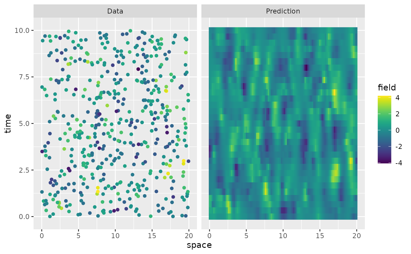
Setting up a data frame
To estimate the model parameters based on this data, we can use the
our rspde_lme function or our inlabru
implementation. For this, we collect the data in a data frame, that also
contains the spatial locations and the time points.
df_1d <- data.frame(y = as.matrix(Y), space = obs.loc$x, time = obs.loc$t)Let us create a mesh for the spatial and temporal domains for the model fitting:
mesh_1d_time <- fmesher::fm_mesh_1d(t)
mesh_1d_space <- fmesher::fm_mesh_1d(s)
Parameter estimation
rspde_lme implementation
We begin by creating an rspde operator:
op_lme1d <- spacetime.operators(mesh_space = mesh_1d_space, mesh_time = mesh_1d_time, alpha = 1, beta = 1)We now fit the model:
res <- rspde_lme(y ~ 1, loc = "space", loc_time = "time", data = df_1d, model = op_lme1d, parallel = TRUE)In the call, y~1 indicates that we also want to estimate
a mean value of the model, and the arguments loc and
loc_time provide the names of the spatial and temporal
coordinates in the data frame. Let us see a summary of the fitted
model:
summary(res)
#>
#> Latent model - Spatio-temporal with alpha =  1 , beta =  1
#>
#> Call:
#> rspde_lme(formula = y ~ 1, loc = "space", loc_time = "time",
#>     data = df_1d, model = op_lme1d, parallel = TRUE)
#>
#> Fixed effects:
#>             Estimate Std.error z-value Pr(>|z|)
#> (Intercept)  0.01225   0.05987   0.205    0.838
#>
#> Random effects:
#>               Estimate Std.error z-value
#> kappa          4.70309   0.38170  12.322
#> sigma          9.06735   1.11125   8.160
#> gamma          0.10761   0.01969   5.465
#> rho            1.03043   0.04652  22.150
#> alpha (fixed)  1.00000        NA      NA
#> beta (fixed)   1.00000        NA      NA
#>
#> Measurement error:
#>          Estimate Std.error z-value
#> std. dev 0.013992  0.008174   1.712
#> ---
#> Signif. codes:  0 '***' 0.001 '**' 0.01 '*' 0.05 '.' 0.1 ' ' 1
#>
#> Log-Likelihood:  -366.9571
#> Number of function calls by 'optim' = 50
#> Optimization method used in 'optim' = L-BFGS-B
#>
#> Time used to:     fit the model =  23.79371 secs
#>   set up the parallelization = 5.25175 secs
Let us compare the estimated results with the true values:
results <- data.frame(
  kappa = c(kappa, res$coeff$random_effects[1]),
  sigma = c(sigma, res$coeff$random_effects[2]),
  gamma = c(gamma, res$coeff$random_effects[3]),
  rho = c(rho_1d, res$coeff$random_effects[4]),
  sigma.e = c(sigma.e, res$coeff$measurement_error),
  intercept = c(0, res$coeff$fixed_effects),
  row.names = c("True", "Estimate")
)

print(results)
#>             kappa     sigma     gamma     rho    sigma.e  intercept
#> True     5.000000 10.000000 0.1000000 1.00000 0.01000000 0.00000000
#> Estimate 4.703093  9.067346 0.1076121 1.03043 0.01399155 0.01225038
Finally, we can also do prediction based on the fitted model as
pred.data <- data.frame(x = rep(s, length(t)), t = rep(t, each = length(s)))
pred <- predict(res, newdata = pred.data, loc = "x", time = "t")
data.df <- data.frame(space = obs.loc$x, time = obs.loc$t, field = Y, type = "Data")
krig.df <- data.frame(
  space = rep(s, length(t)), time = rep(t, each = length(s)),
  field = as.vector(pred$mean), type = "Prediction"
)
df_plot <- rbind(data.df, krig.df)
ggplot(df_plot) +
  aes(x = space, y = time, fill = field) +
  facet_wrap(~type) +
  geom_raster(data = krig.df) +
  geom_point(
    data = data.df, aes(colour = field),
    show.legend = FALSE
  ) +
  scale_fill_viridis() +
  scale_colour_viridis()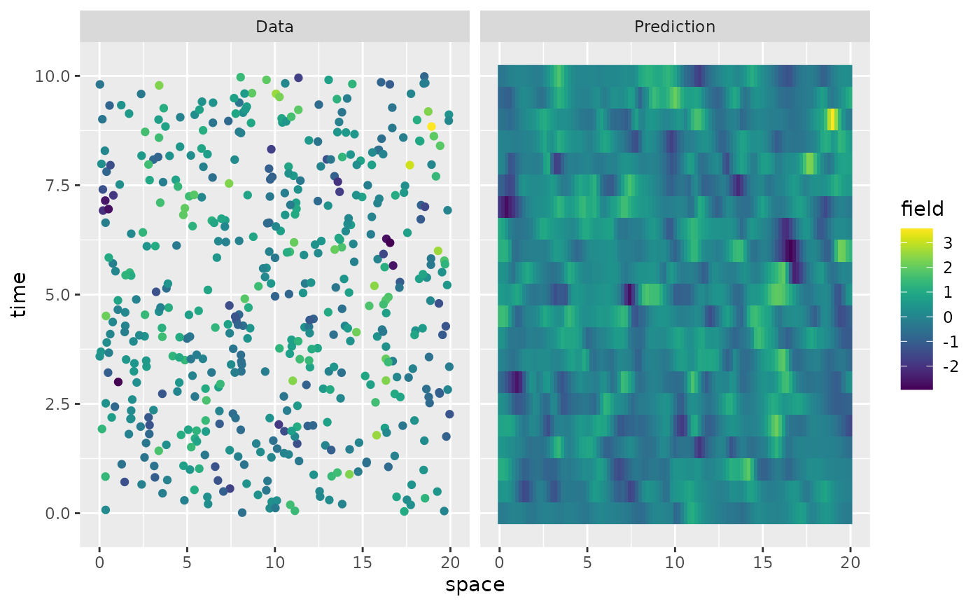
inlabru Implementation
Let us now fit the model using our inlabru
implementation. We start by creating the model object with the
rspde.spacetime() function:
library(inlabru)
#> Loading required package: fmesher
st_bru <- rspde.spacetime(mesh_space = mesh_1d_space, mesh_time = mesh_1d_time, alpha = 1, beta = 1)
We now create the model component, which requires the user to pass
the index as a list containing the elements space with the
spatial indices and time with the temporal indices:
cmp <- y ~ -1 + Intercept(1) + field(list(space = space, time = time), model = st_bru)We are now in a position to fit the model:
Let us now compare the estimated results (the means of the parameters) with the true values:
param_st_1d <- transform_parameters_spacetime(
  bru_fit$summary.hyperpar$mean[2:5],
  st_bru
)

results <- data.frame(
  kappa = c(kappa, param_st_1d[[1]]),
  sigma = c(sigma, param_st_1d[[2]]),
  gamma = c(gamma, param_st_1d[[3]]),
  rho = c(rho_1d, param_st_1d[[4]]),
  sigma.e = c(sigma.e, sqrt(1 / bru_fit$summary.hyperpar$mean[1])),
  intercept = c(0, bru_fit$summary.fixed$mean),
  row.names = c("True", "Estimate")
)

print(results)
#>             kappa     sigma     gamma      rho    sigma.e  intercept
#> True     5.000000 10.000000 0.1000000 1.000000 0.01000000 0.00000000
#> Estimate 4.677085  9.123076 0.1061707 1.191519 0.01005917 0.01271066
A spatial example
Let us now illustrate how to implement a spatial version. We start by
creating a region of interest and a spatial mesh using the
fmesher package:
library(fmesher)
n_loc <- 1000
loc_2d_mesh <- matrix(runif(n_loc * 2), n_loc, 2)
mesh_2d <- fm_mesh_2d(
  loc = loc_2d_mesh,
  cutoff = 0.07,
  max.edge = c(0.2, 0.6)
)
plot(mesh_2d, main = "")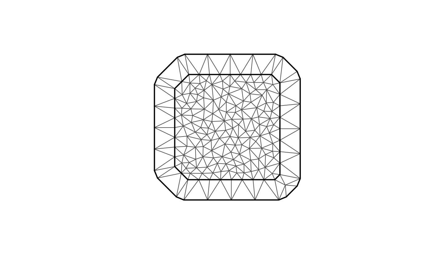
We now proceed as previously by defining a temporal region and the model
t <- seq(from = 0, to = 10, length.out = 11)
kappa <- 9.9
sigma <- 29
gamma <- 0.11
rho_2d <- c(0.2, 0.3)
alpha <- 1
beta <- 1

op <- spacetime.operators(
  mesh_space = mesh_2d, time_loc = t,
  kappa = kappa, sigma = sigma, alpha = alpha,
  beta = beta, rho = rho_2d, gamma = gamma
)
op$plot_covariances(s.ind = 100, t.ind = 5, t.shift = c(-2, 0, 2))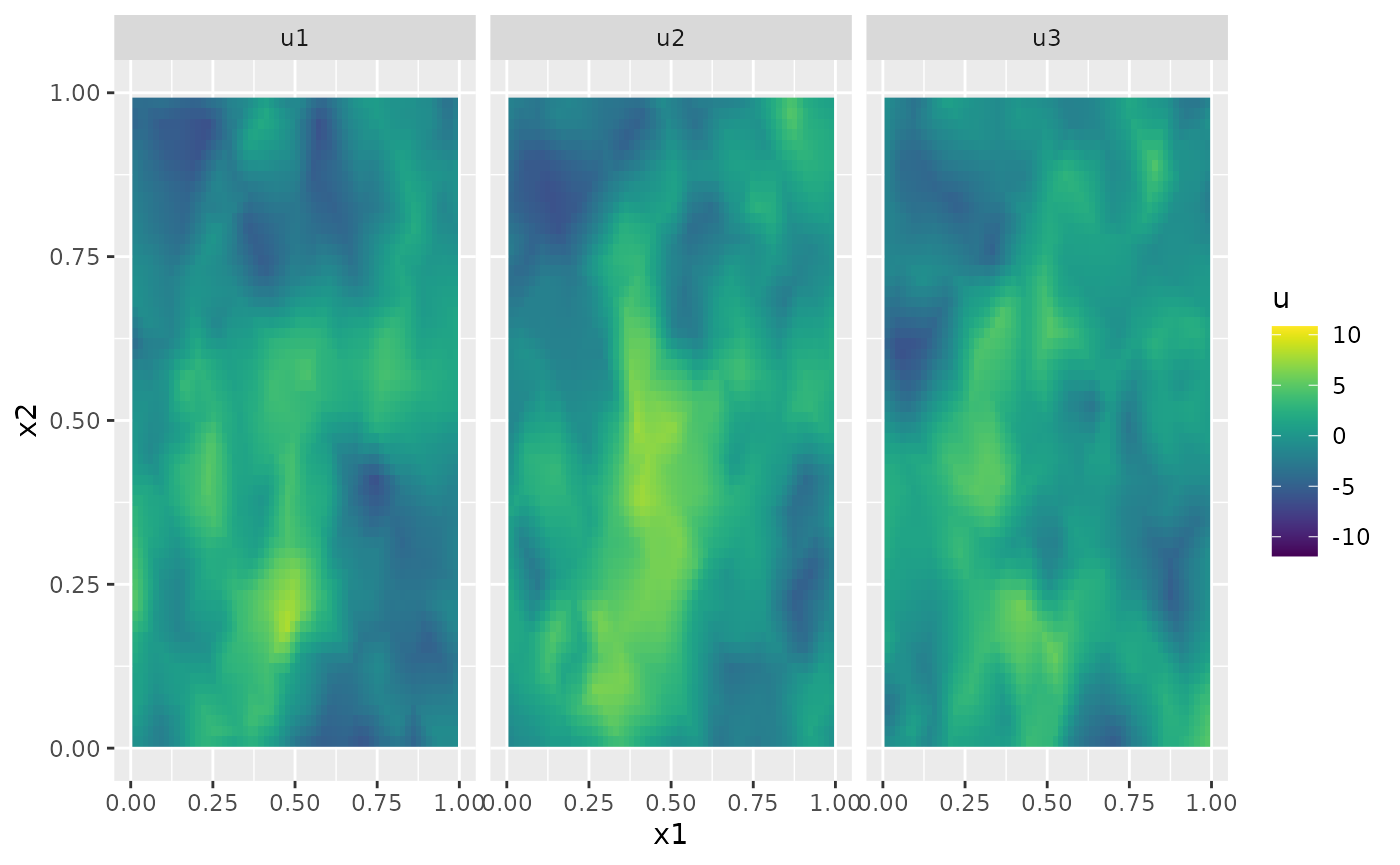
#> TableGrob (2 x 1) "arrange": 2 grobs
#>   z     cells    name           grob
#> 1 1 (1-1,1-1) arrange gtable[layout]
#> 2 2 (2-2,1-1) arrange gtable[layout]
#> TableGrob (2 x 1) "arrange": 2 grobs
#>   z     cells    name           grob
#> 1 1 (1-1,1-1) arrange gtable[layout]
#> 2 2 (2-2,1-1) arrange gtable[layout]
The spacetime.operators object has a
plot_covariances method which can be used to vizualise
marginal spatial and temporal covariances. The function takes as input
t.ind which is the index of the location in the time
discretization to plot the marginal spatial covariance for, and an input
s.ind which is the index of the location in the space
discretization to show the marginal temporal covariance for. It further
takes an input t.shift which can be used to plot
covariances
,
where
is t[t.ind] and
is t[t.ind + t.shift]. For example
We can simulate from the model using simulate():
u <- simulate(op)Let us plot the simulation for a few time points
proj <- fm_evaluator(mesh_2d, dims = c(100, 100))
U <- matrix(u, nrow = mesh_2d$n, ncol = length(t))
field1 <- fm_evaluate(proj, field = as.vector(U[, 2]))
field2 <- fm_evaluate(proj, field = as.vector(U[, 3]))
field3 <- fm_evaluate(proj, field = as.vector(U[, 4]))

field1.df <- data.frame(
  x1 = proj$lattice$loc[, 1], x2 = proj$lattice$loc[, 2],
  u = as.vector(field1), type = "u1"
)
field2.df <- data.frame(
  x1 = proj$lattice$loc[, 1], x2 = proj$lattice$loc[, 2],
  u = as.vector(field2), type = "u2"
)
field3.df <- data.frame(
  x1 = proj$lattice$loc[, 1], x2 = proj$lattice$loc[, 2],
  u = as.vector(field3), type = "u3"
)
field.df <- rbind(field1.df, field2.df, field3.df)
ggplot(field.df) +
  aes(x = x1, y = x2, fill = u) +
  facet_wrap(~type) +
  geom_raster() +
  xlim(0, 1) +
  ylim(0, 1) +
  scale_fill_viridis()
#> Warning: Removed 18468 rows containing missing values or values outside the scale range
#> (`geom_raster()`).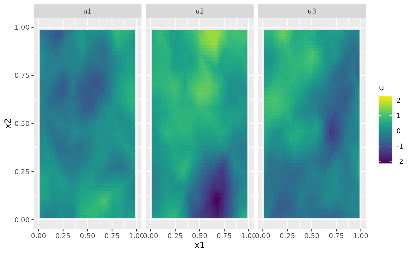
We now generate the observations as , where is Gaussian measurement noise.
Setting up a data frame
To estimate the model parameters based on this data, we can use the
rspde_lme function. For this, we collect the data in a data
frame, that also contanis the spatial locations, and we fit the
model:
df_2d <- data.frame(Y = as.matrix(Y), x = obs.loc$x, y = obs.loc$y, t = obs.loc$t)Let us also create spatial and temporal meshes for the model fitting:
mesh_2d_spatial <- fm_mesh_2d(
  loc = df_2d[, c("x", "y")],
  cutoff = 0.07,
  max.edge = c(0.2, 0.6)
)

mesh_2d_time <- fmesher::fm_mesh_1d(t)
rspde_lme implementation
We begin by creating an rspde operator:
op_lme2d <- spacetime.operators(mesh_space = mesh_2d_spatial, mesh_time = mesh_2d_time, alpha = 1, beta = 1)Let us now fit the model:
res_2d <- rspde_lme(Y ~ 1, loc = c("x", "y"), loc_time = "t", data = df_2d, model = op_lme2d, parallel = TRUE)Let us see a summary of the fitted model:
summary(res_2d)
#>
#> Latent model - Spatio-temporal with alpha =  1 , beta =  1
#>
#> Call:
#> rspde_lme(formula = Y ~ 1, loc = c("x", "y"), loc_time = "t",
#>     data = df_2d, model = op_lme2d, parallel = TRUE)
#>
#> Fixed effects:
#>             Estimate Std.error z-value Pr(>|z|)
#> (Intercept)  0.03702   0.04815   0.769    0.442
#>
#> Random effects:
#>               Estimate Std.error z-value
#> kappa          9.71690   0.74406  13.059
#> sigma         11.91772   6.46225   1.844
#> gamma          0.06230   0.03416   1.824
#> rho            0.07952   0.60347   0.132
#> rho2           0.12814   0.76728   0.167
#> alpha (fixed)  1.00000        NA      NA
#> beta (fixed)   1.00000        NA      NA
#>
#> Measurement error:
#>          Estimate Std.error z-value
#> std. dev  0.04683   0.10797   0.434
#> ---
#> Signif. codes:  0 '***' 0.001 '**' 0.01 '*' 0.05 '.' 0.1 ' ' 1
#>
#> Log-Likelihood:  149.8674
#> Number of function calls by 'optim' = 81
#> Optimization method used in 'optim' = L-BFGS-B
#>
#> Time used to:     fit the model =  2.62917 mins
#>   set up the parallelization = 5.81546 secs
Let us compare the estimated results with the true values:
results <- data.frame(
  kappa = c(kappa, res_2d$coeff$random_effects[1]),
  sigma = c(sigma, res_2d$coeff$random_effects[2]),
  gamma = c(gamma, res_2d$coeff$random_effects[3]),
  rho_1 = c(rho_2d[1], res_2d$coeff$random_effects[4]),
  rho_2 = c(rho_2d[2], res_2d$coeff$random_effects[5]),
  sigma.e = c(sigma.e, res_2d$coeff$measurement_error),
  intercept = c(0, res_2d$coeff$fixed_effects),
  row.names = c("True", "Estimate")
)

print(results)
#>           kappa    sigma      gamma      rho_1     rho_2    sigma.e  intercept
#> True     9.9000 29.00000 0.11000000 0.20000000 0.3000000 0.01000000 0.00000000
#> Estimate 9.7169 11.91772 0.06229692 0.07952026 0.1281441 0.04683419 0.03702228
Let us now use our inlabru implementation. We first
define the model.
st_bru_field <- rspde.spacetime(
  mesh_space = mesh_2d_spatial,
  mesh_time = mesh_2d_time, alpha = 1, beta = 1
)
Now, the component:
We are now in a position to fit the model:
Let us now compare the estimated results (the means of the parameters) with the true values:
param_st <- transform_parameters_spacetime(
  bru_fit_field$summary.hyperpar$mean[2:6],
  st_bru_field
)

results <- data.frame(
  kappa = c(kappa, param_st[[1]]),
  sigma = c(sigma, param_st[[2]]),
  gamma = c(gamma, param_st[[3]]),
  rho_1 = c(rho_2d[1], param_st[[4]]),
  rho_2 = c(rho_2d[2], param_st[[5]]),
  sigma.e = c(sigma.e, sqrt(1 / bru_fit_field$summary.hyperpar$mean[1])),
  intercept = c(0, bru_fit_field$summary.fixed$mean),
  row.names = c("True", "Estimate")
)

print(results)
#>              kappa        sigma        gamma        rho_1        rho_2
#> True     9.9000000 2.900000e+01 1.100000e-01  0.200000000  0.300000000
#> Estimate 0.3009676 3.848025e-05 8.723392e-09 -0.003454795 -0.004320446
#>               sigma.e intercept
#> True     0.0100000000 0.0000000
#> Estimate 0.0005200932 0.4928725
Fit with bounded_rho = FALSE
In cases where the estimated value of
approaches the upper bound (available in st_bru$bound_rho),
the model can be re-fitted with bounded_rho = FALSE. This
removes the bounding constraint on
,
which can lead to a better fit but may introduce numerical instability.
Below, we demonstrate this for both the 1D and spatial examples.
1D Example with bounded_rho = FALSE
Let us first start with the rspde_lme() example. We will
use the previous fit as a starting point for the new fit to improve the
convergence of the optimization.
op_1d_unbounded <- spacetime.operators(
  space_loc = s_1d, time_loc = t_1d,
  alpha = 1, beta = 1,
  bounded_rho = FALSE
)

res_unbounded <- rspde_lme(y ~ 1,
  loc = "space", loc_time = "time",
  data = df_1d, model = op_1d_unbounded, parallel = TRUE,
  previous_fit = res
)

results <- data.frame(
  kappa = c(kappa, res_unbounded$coeff$random_effects[1]),
  sigma = c(sigma, res_unbounded$coeff$random_effects[2]),
  gamma = c(gamma, res_unbounded$coeff$random_effects[3]),
  rho = c(rho_1d, res_unbounded$coeff$random_effects[4]),
  sigma.e = c(sigma.e, res_unbounded$coeff$measurement_error),
  intercept = c(0, res_unbounded$coeff$fixed_effects),
  row.names = c("True", "Estimate")
)

print(results)
#>             kappa     sigma     gamma     rho   sigma.e  intercept
#> True     9.900000 29.000000 0.1100000 1.00000 0.0100000 0.00000000
#> Estimate 4.703064  9.066892 0.1076067 1.03032 0.0139923 0.01228339
Now, the inlabru implementation:
### Fit with bounded_rho = FALSE
st_bru_unbounded <- rspde.spacetime(
  space_loc = s_1d, time_loc = t_1d, alpha = 1,
  beta = 1, bounded_rho = FALSE
)

### Fitting the Model
cmp_unbounded <- y ~ -1 + Intercept(1) + field(list(space = space, time = time),
  model = st_bru_unbounded
)

bru_fit_unbounded <- bru(cmp_unbounded, data = df_1d, options = list(num.threads = "1:1", verbose = TRUE))

### Extract and Compare Results
param_unbounded <- transform_parameters_spacetime(
  bru_fit_unbounded$summary.hyperpar$mean[2:5],
  st_bru_unbounded
)

results_unbounded <- data.frame(
  kappa = c(kappa, param_unbounded$kappa),
  sigma = c(sigma, param_unbounded$sigma),
  gamma = c(gamma, param_unbounded$gamma),
  rho = c(rho_1d, param_unbounded$rho),
  sigma.e = c(sigma.e, sqrt(1 / bru_fit_unbounded$summary.hyperpar$mean[1])),
  intercept = c(0, bru_fit_unbounded$summary.fixed$mean),
  row.names = c("True", "Estimate")
)

print(results_unbounded)
#>             kappa     sigma      gamma      rho     sigma.e  intercept
#> True     9.900000 29.000000 0.11000000 1.000000 0.010000000 0.00000000
#> Estimate 5.026244  9.082655 0.08955354 1.418052 0.007723455 0.01239866