Rational approximations without finite element approximations

Introduction

For models in one dimension, we can perform rational approximations without finite elements. This enables us to provide computationally efficient approximations of Gaussian processes with Mat'ern covariance functions, without having to define finite element meshes, and without having boundary effects due to the boundary conditions that are usually required. In this vignette we will introduce these methods.

We begin by loading the rSPDE package:

library(rSPDE)

## Error in get(paste0(generic, ".", class), envir = get_method_env()) : 
##   object 'type_sum.accel' not found

Assume that we want to define a model on the interval $[0,1]$ , which we want to evaluate at some locations

s <- seq(from = 0, to = 1, length.out = 101)

We can now use matern.rational() to construct a rational SPDE approximation of order $m=2$ for a Gaussian random field with a Matérn covariance function on the interval.

kappa <- 20
sigma <- 2
nu <- 0.8
r <- sqrt(8*nu)/kappa #range parameter
op_cov <- matern.rational(loc = s, nu = nu, range = r, sigma = sigma, m = 2, parameterization = "matern")

The object op_cov contains the information needed for evaluating the approximation. Note, however, that the approximation is invariant to the locations loc, and they are only supplied to indicate where we want to evaluate it.

To evaluate the accuracy of the approximation, let us compute the covariance function between the process at $s=0$ and all other locations in s and compare with the true Matérn covariance function. The covariances can be calculated by using the covariance() method.

c_cov.approx <- op_cov$covariance(ind = 1)
c.true <- matern.covariance(abs(s[1] - s), kappa, nu, sigma)

The covariance function and the error compared with the Matérn covariance are shown in the following figure.

opar <- par(
  mfrow = c(1, 2), mgp = c(1.3, 0.5, 0),
  mar = c(2, 2, 0.5, 0.5) + 0.1
)
plot(s, c.true,
  type = "l", ylab = "C(|s-0.5|)", xlab = "s", ylim = c(0, 5),
  cex.main = 0.8, cex.axis = 0.8, cex.lab = 0.8
)
lines(s, c_cov.approx, col = 2)
legend("topright",
  bty = "n",
  legend = c("Matérn", "Rational"),
  col = c("black", "red"),
  lty = rep(1, 2), ncol = 1,
  cex = 0.8
)

plot(s, c.true - c_cov.approx,
  type = "l", ylab = "Error", xlab = "s",
  cex.main = 0.8, cex.axis = 0.8, cex.lab = 0.8
)
par(opar)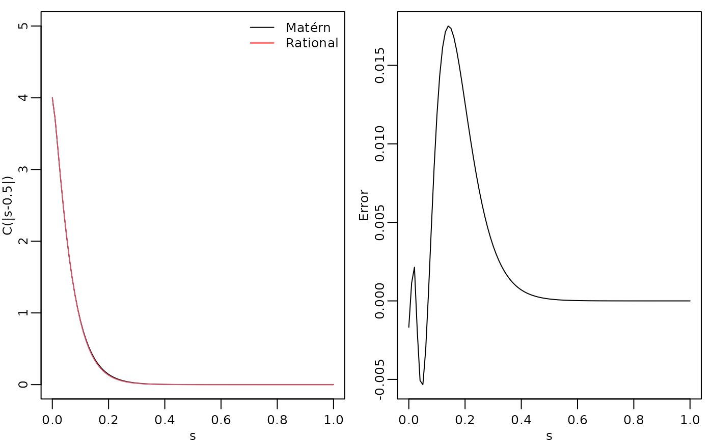

To improve the approximation we can increase the order of the approximation, by increasing $m$ . Let us, for example, compute the approximation with $m=1,\ldots,4$ .

errors <- rep(0, 4)
for (i in 1:4) {
  op_cov_i <- matern.rational(loc = s, range = r, sigma = sigma, nu = nu,
                            m = i, parameterization = "matern")
  errors[i] <- norm(c.true - op_cov_i$covariance(ind = 1))
}
print(errors)

## [1] 1.36208052 0.29200800 0.07907210 0.02597968

We see that the error decreases very fast when we increase $m$ from $1$ to $4$ .

Simulation

We can simulate from the constructed model using the simulate() method. To such an end we simply apply the simulate() method to the object returned by the matern.operators() function:

u <- simulate(op_cov)
plot(s, u, type = "l")

If we want replicates, we simply set the argument nsim to the desired number of replicates. For instance, to generate two replicates of the model, we simply do:

u.rep <- simulate(op_cov, nsim = 2)

Inference

There is built-in support for computing log-likelihood functions and performing kriging prediction in the rSPDE package. To illustrate this, we use the simulation to create some noisy observations of the process. For this, we first construct the observation matrix linking the FEM basis functions to the locations where we want to simulate. We first randomly generate some observation locations and then construct the matrix.

set.seed(1)
n.obs <- 100
obs.loc <- sort(runif(n.obs))

We now generate the observations as $Y_i = 2 - x1 + u(s_i) + \varepsilon_i$ , where $\varepsilon_i \sim N(0,\sigma_e^2)$ is Gaussian measurement noise, $x1$ is a covariate giving the observation location. We will assume that the latent process has a Matérn covariance with $\kappa=20, \sigma=1.3$ and $\nu=0.8$ :

n.rep <- 10
kappa <- 20
sigma <- 1.3
nu <- 0.8
r <- sqrt(8*nu)/kappa
op_cov <- matern.rational(loc = obs.loc, nu = nu, range = r, sigma = sigma, m = 2, 
                          parameterization = "matern")

u <- matrix(simulate(op_cov, n = n.rep), ncol = n.rep)

sigma.e <- 0.3

x1 <- obs.loc

Y <- matrix(rep(2 - x1, n.rep), ncol = n.rep) + u + sigma.e * matrix(rnorm(n.obs*n.rep), ncol = n.rep)
repl <- rep(1:n.rep, each = n.obs)
df_data <- data.frame(y = as.vector(Y), loc = rep(obs.loc, n.rep), 
                      x1 = rep(x1, n.rep), repl = repl)

Let us create a new object to fit the model:

op_cov_est <- matern.rational(loc = obs.loc, m = 2)

Let us now fit the model. To this end we will use the rspde_lme() function:

fit <- rspde_lme(y~x1, model = op_cov_est,
                 repl = repl, data = df_data, loc = "loc",
                 parallel = TRUE)

Here is the summary:

summary(fit)

## 
## Latent model - Whittle-Matern
## 
## Call:
## rspde_lme(formula = y ~ x1, loc = "loc", data = df_data, model = op_cov_est, 
##     repl = repl, parallel = TRUE)
## 
## Fixed effects:
##             Estimate Std.error z-value Pr(>|z|)    
## (Intercept)   2.0140    0.2957   6.811 9.68e-12 ***
## x1           -1.1955    0.4970  -2.406   0.0161 *  
## 
## Random effects:
##       Estimate Std.error z-value
## alpha  1.41381   0.10804   13.09
## tau    0.02485   0.01249    1.99
## kappa 21.51541   3.79491    5.67
## 
## Random effects (Matern parameterization):
##       Estimate Std.error z-value
## nu     0.91381   0.10804   8.458
## sigma  1.41331   0.08741  16.168
## range  0.12567   0.01120  11.220
## 
## Measurement error:
##          Estimate Std.error z-value
## std. dev  0.29204   0.01444   20.23
## ---
## Signif. codes:  0 '***' 0.001 '**' 0.01 '*' 0.05 '.' 0.1 ' ' 1 
## 
## Log-Likelihood:  -876.9438 
## Number of function calls by 'optim' = 61
## Optimization method used in 'optim' = L-BFGS-B
## 
## Time used to:     fit the model =  2.84639 mins 
##   set up the parallelization = 2.33818 secs

Let us compare with the true values and compare the time:

print(data.frame(
  sigma = c(sigma, fit$matern_coeff$random_effects[2]), 
  range = c(r, fit$matern_coeff$random_effects[3]),
  nu = c(nu, fit$matern_coeff$random_effects[1]),
  row.names = c("Truth", "Estimates")
))

##              sigma     range       nu
## Truth     1.300000 0.1264911 0.800000
## Estimates 1.413308 0.1256677 0.913812

# Total time (time to fit plus time to set up the parallelization)
total_time <- fit$fitting_time + fit$time_par
print(total_time)

## Time difference of 173.122 secs

Kriging

Finally, we compute the kriging prediction of the process $u$ at the locations in s based on these observations.

Let us create the data.frame with locations in which we want to obtain the predictions. Observe that we also must provide the values of the covariates.

s <- seq(from = 0, to = 1, length.out = 100)
df_pred <- data.frame(loc = s, x1 = s)

We can now perform kriging with the predict() method. For example, to predict at the locations for the first replicate:

u.krig <- predict(fit, newdata = df_pred, loc = "loc", which_repl = 1)

The simulated process, the observed data, and the kriging prediction are shown in the following figure.

opar <- par(mgp = c(1.3, 0.5, 0), mar = c(2, 2, 0.5, 0.5) + 0.1)
plot(obs.loc, Y[,1],
  ylab = "u(s)", xlab = "s",
  ylim = c(min(c(min(u), min(Y))), max(c(max(u), max(Y)))),
  cex.main = 0.8, cex.axis = 0.8, cex.lab = 0.8
)
lines(s, u.krig$mean, col = 2)
par(opar)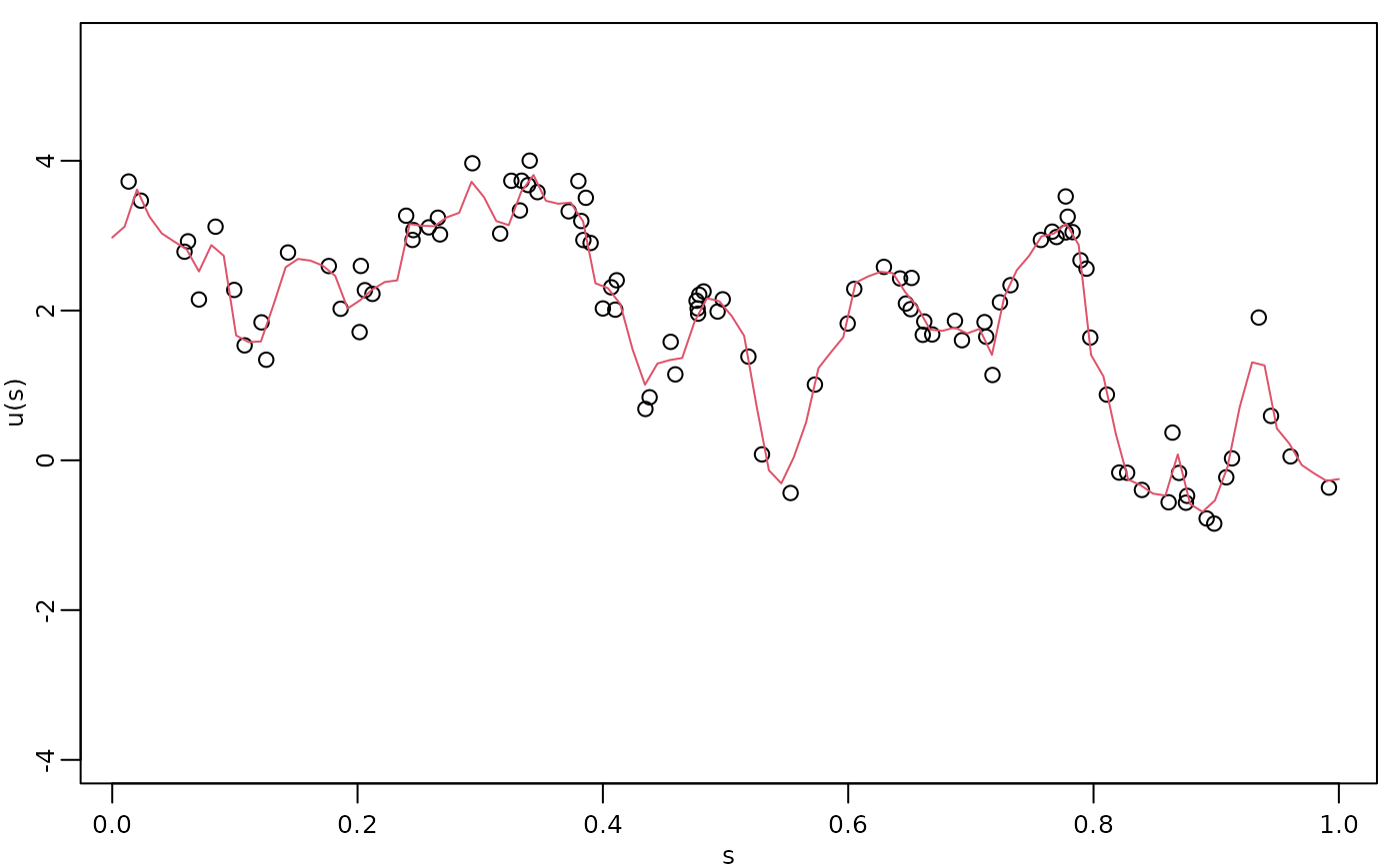

We can also use the augment() function and pipe the results into a plot:

library(ggplot2)
library(dplyr)

augment(fit, newdata = df_pred, loc = "loc", which_repl = 1) %>% ggplot() + 
                aes(x = loc, y = .fitted) +
                geom_line(col="red") + 
                geom_point(data = df_data[df_data$repl==1,], aes(x = loc, y=y))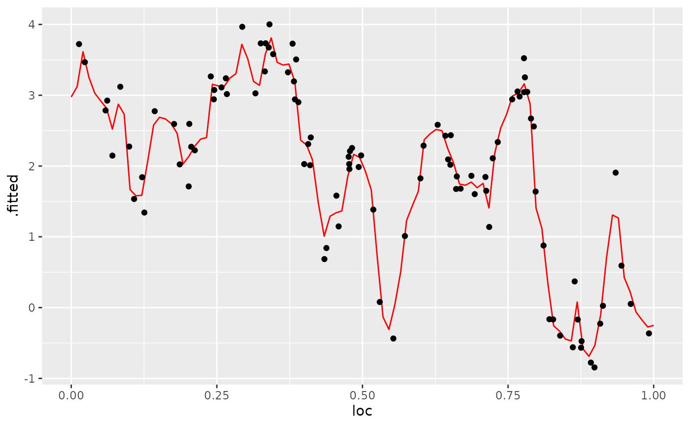

Using the models in `INLA`

The inla implementation of the models is found in the rspde.matern1d function. To test it, let us simulate some data again.

sigma <- 1
nu <- 0.8
sigma.e <- 0.1
n.obs <- 1000
r <- 1
s <- seq(from = 0, to = 5, length.out = n.obs)
op_cov <- matern.rational(loc = s, nu = nu, range = r, sigma = sigma, m = 1, parameterization = "matern")
u <- simulate(op_cov)
Y <- u + sigma.e * rnorm(n.obs)
plot(s, u, type = "l")
points(s,Y,col=2)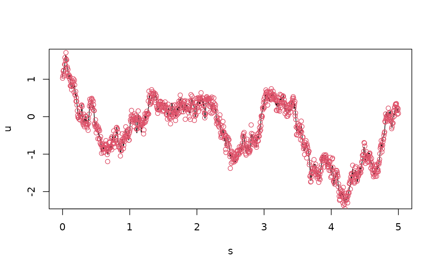

We can now specify the model and fit it to the data using inla. In the following code, we fix the smoothness parameter to 0.5. In this case, it will not be estimated in inla. By removing the specification of nu in the rspde.matern1d call, it is assumed to be free and will be estimated from data. Note that the A matrix and the index vector needed by inla are pre-computed in the function. The default name of the model component (set in the index vector) is field.

library(INLA)

## This is INLA_24.12.11 built 2024-12-11 19:58:26 UTC.
##  - See www.r-inla.org/contact-us for how to get help.
##  - List available models/likelihoods/etc with inla.list.models()
##  - Use inla.doc(<NAME>) to access documentation

inla_model <- rspde.matern1d(loc = s, nu = 0.5)
st.dat <- inla.stack(data = list(y = as.vector(Y)), A = inla_model$A, effects = inla_model$index)
res <- inla(y ~ -1 + f(field, model = inla_model), 
        data = inla.stack.data(st.dat),
        family = "gaussian",
        control.predictor = list(A = inla.stack.A(st.dat)))

Let us look at some summaries of the fit:

result_fit <- rspde.result(res, "field", inla_model, parameterization = "matern") 
summary(result_fit)

##            mean       sd 0.025quant 0.5quant 0.975quant     mode
## std.dev 1.02833 0.343709   0.574486 0.950778    1.88264 0.836471
## range   2.96527 2.377920   0.762279 2.271220    9.26631 1.549250

posterior_df_fit <- gg_df(result_fit)

ggplot(posterior_df_fit) + geom_line(aes(x = x, y = y)) + 
facet_wrap(~parameter, scales = "free") + labs(y = "Density")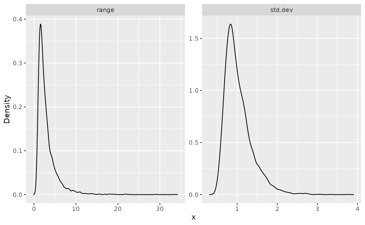

Using the models in `inlabru`

Let us now fit the following model using our inlabru implementation. In this case, we will estimate nu.

sigma <- 1
nu <- 0.8
sigma.e <- 0.1
n.obs <- 251
r <- 1
s <- seq(from = 0, to = 5, length.out = n.obs)
op_cov <- matern.rational(loc = s, nu = nu, range = r, sigma = sigma, m = 1, parameterization = "matern")
u <- simulate(op_cov)
Y <- u + sigma.e * rnorm(n.obs)

We need to create a data.frame with the response variables and locations:

df_bru <- data.frame(y = Y, loc = s)

We now create the model object, without specifying nu:

bru_model <- rspde.matern1d(loc = s)

Finally, we can load the inlabru package, create the model component, and fit the model:

library(inlabru)

## Loading required package: fmesher

cmp <- y ~ -1 + Intercept(1) + field(loc, model = bru_model)
bru_fit <- bru(cmp, data = df_bru, options = list(num.threads = "1:1"))

Let us, again, look at the summaries of the fit:

result_fit <- rspde.result(bru_fit, "field", bru_model, parameterization = "matern") 
summary(result_fit)

##             mean       sd 0.025quant 0.5quant 0.975quant     mode
## std.dev 1.070490 0.322368   0.595001 1.016860    1.82162 0.925755
## range   0.809706 0.264479   0.411487 0.772491    1.44312 0.707675
## nu      0.974084 0.199441   0.600189 0.968805    1.37202 0.948629

Kriging with the inlabru implementation

We will now do prediction with the previous model. To this end, we start by creating the data.frame containing the locations in which we want to do prediction:

s_pred <- seq(from = 0, to = 5, length.out = 1001)
df_pred <- data.frame(loc = s_pred)

Now, first observe that we cannot directly use inlabru’s predict method:

pred <- predict(bru_fit, newdata = df_pred, formula = ~ Intercept + field)

## Error in match_with_tolerance(input, loc): Error: The input location 0.0050000000 is not present in the original locations used to create the model object.

Indeed, it complained that we are trying to obtain predictions at locations that were not used to create the model object. However, we can obtain predictions using our modified predict method, in which we need to pass the components and well as the model:

pred <- predict(bru_model, cmp, bru_fit, newdata = df_pred, formula = ~ Intercept + field)

David Bolin and Alexandre B. Simas

Created: 2024-07-20. Last modified: 2024-12-20.

Introduction

Simulation

Inference

Kriging

Using the models in `INLA`

Using the models in `inlabru`

Kriging with the inlabru implementation

References

Rational approximations without finite element approximations

David Bolin and Alexandre B. Simas

Created: 2024-07-20. Last modified: 2024-12-20.

Introduction

Simulation

Inference

Kriging

Using the models in INLA

Using the models in inlabru

Kriging with the inlabru implementation

References

Using the models in `INLA`

Using the models in `inlabru`