inlabru implementation of the rational SPDE approach

Introduction

In this vignette we will present the inlabru implementation of the covariance-based rational SPDE approach. For further technical details on the covariance-based approach, see the Rational approximation with the rSPDE package vignette and Bolin, Simas, and Xiong (2023).

We begin by providing a step-by-step illustration on how to use our implementation. To this end we will consider a real world data set that consists of precipitation measurements from the Paraná region in Brazil.

After the initial model fitting, we will show how to change some parameters of the model. In the end, we will also provide an example in which we have replicates.

The examples in this vignette are the same as those in the R-INLA implementation of the rational SPDE approach vignette. As in that case, it is important to mention that one can improve the performance by using the PARDISO solver. Please, go to https://www.pardiso-project.org/r-inla/#license to apply for a license. Also, use inla.pardiso() for instructions on how to enable the PARDISO sparse library.

An example with real data

To illustrate our implementation of rSPDE in inlabru we will consider a dataset available in R-INLA. This data has also been used to illustrate the SPDE approach, see for instance the book Advanced Spatial Modeling with Stochastic Partial Differential Equations Using R and INLA and also the vignette Spatial Statistics using R-INLA and Gaussian Markov random fields. See also Lindgren, Rue, and Lindström (2011) for theoretical details on the standard SPDE approach.

The data consist of precipitation measurements from the Paraná region in Brazil and were provided by the Brazilian National Water Agency. The data were collected at 616 gauge stations in Paraná state, south of Brazil, for each day in 2011.

An rSPDE model for precipitation

We will follow the vignette Spatial Statistics using R-INLA and Gaussian Markov random fields. As precipitation data are always positive, we will assume it is Gamma distributed. R-INLA uses the following parameterization of the Gamma distribution, \[\Gamma(\mu, \phi): \pi (y) = \frac{1}{\Gamma(\phi)} \left(\frac{\phi}{\mu}\right)^{\phi} y^{\phi - 1} \exp\left(-\frac{\phi y}{\mu}\right) .\] In this parameterization, the distribution has expected value \(E(x) = \mu\) and variance \(V(x) = \mu^2/\phi\), where \(1/\phi\) is a dispersion parameter.

In this example \(\mu\) will be modelled using a stochastic model that includes both covariates and spatial structure, resulting in the latent Gaussian model for the precipitation measurements \[\begin{align} y_i\mid \mu(s_i), \theta &\sim \Gamma(\mu(s_i),c\phi)\\ \log (\mu(s)) &= \eta(s) = \sum_k f_k(c_k(s))+u(s)\\ \theta &\sim \pi(\theta) \end{align},\]

where \(y_i\) denotes the measurement taken at location \(s_i\), \(c_k(s)\) are covariates, \(u(s)\) is a mean-zero Gaussian Matérn field, and \(\theta\) is a vector containing all parameters of the model, including smoothness of the field. That is, by using the rSPDE model we will also be able to estimate the smoothness of the latent field.

Examining the data

We will be using inlabru. The inlabru package is available on CRAN and also on GitHub.

We begin by loading some libraries we need to get the data and build the plots.

library(ggplot2)
library(INLA)
library(inlabru)
library(splancs)
library(viridis)

Let us load the data and the border of the region

data(PRprec)
data(PRborder)

The data frame contains daily measurements at 616 stations for the year 2011, as well as coordinates and altitude information for the measurement stations. We will not analyze the full spatio-temporal data set, but instead look at the total precipitation in January, which we calculate as

Y <- rowMeans(PRprec[, 3 + 1:31])

In the next snippet of code, we extract the coordinates and altitudes and remove the locations with missing values.

ind <- !is.na(Y)
Y <- Y[ind]
coords <- as.matrix(PRprec[ind, 1:2])
alt <- PRprec$Altitude[ind]

Let us build a plot for the precipitations:

ggplot() +
  geom_point(aes(
    x = coords[, 1], y = coords[, 2],
    colour = Y
  ), size = 2, alpha = 1) +
  geom_path(aes(x = PRborder[, 1], y = PRborder[, 2])) +
  geom_path(aes(x = PRborder[1034:1078, 1], y = PRborder[
    1034:1078,
    2
  ]), colour = "red") + 
  scale_color_viridis()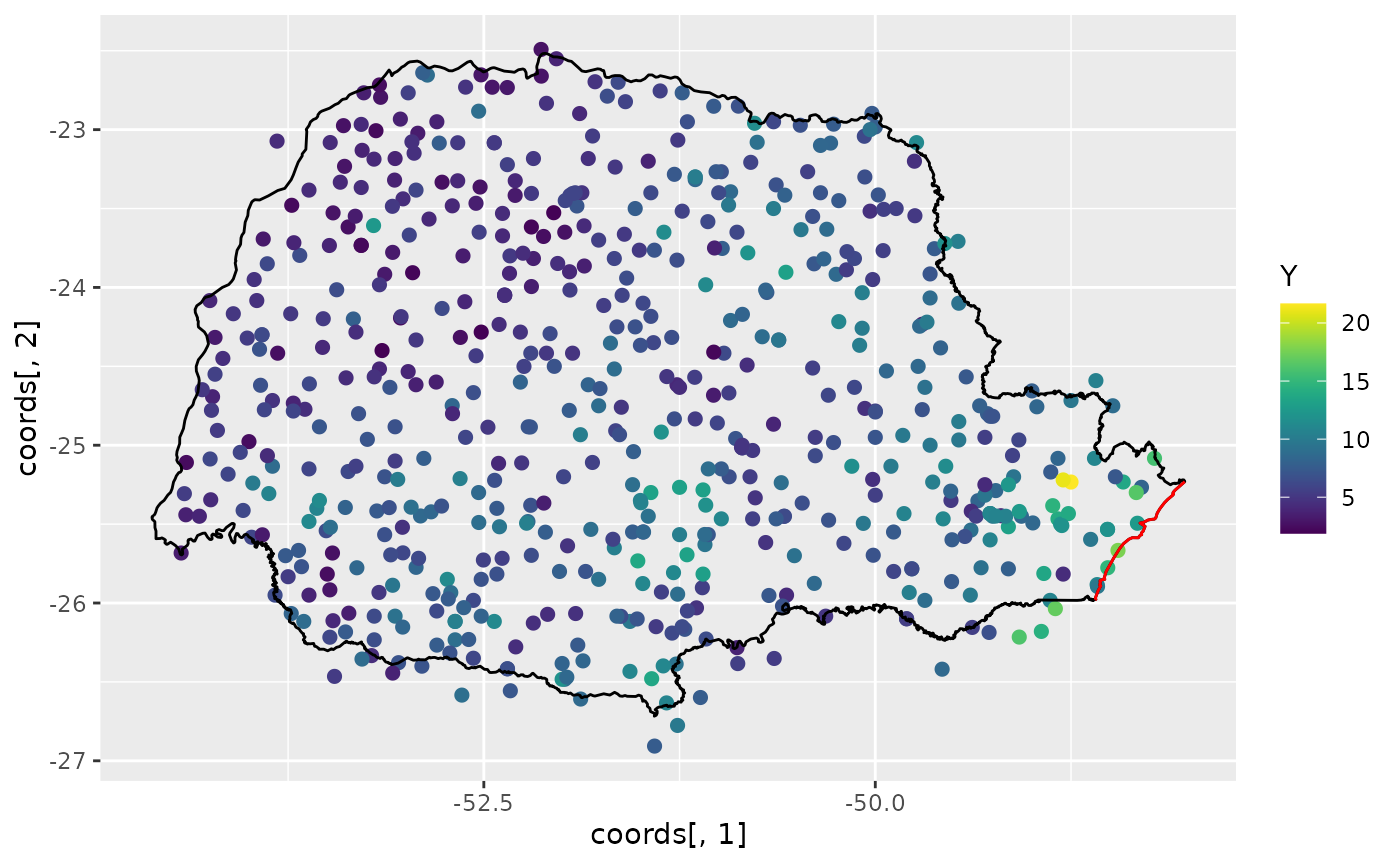

The red line in the figure shows the coast line, and we expect the distance to the coast to be a good covariate for precipitation.

This covariate is not available, so let us calculate it for each observation location:

seaDist <- apply(spDists(coords, PRborder[1034:1078, ],
  longlat = TRUE
), 1, min)

Now, let us plot the precipitation as a function of the possible covariates:

par(mfrow = c(2, 2))
plot(coords[, 1], Y, cex = 0.5, xlab = "Longitude")
plot(coords[, 2], Y, cex = 0.5, xlab = "Latitude")
plot(seaDist, Y, cex = 0.5, xlab = "Distance to sea")
plot(alt, Y, cex = 0.5, xlab = "Altitude")

par(mfrow = c(1, 1))

Creating the rSPDE model

To use the inlabru implementation of the rSPDE model we need to load the functions:

library(rSPDE)

To create a rSPDE model, one would the rspde.matern() function in a similar fashion as one would use the inla.spde2.matern() function.

Mesh

We can use fm_mesh_2d() function from the fmesher package for creating the mesh. Let us create a mesh which is based on a non-convex hull to avoid adding many small triangles outside the domain of interest:

library(fmesher)

prdomain <- fm_nonconvex_hull(coords, -0.03, -0.05, resolution = c(100, 100))
prmesh <- fm_mesh_2d(boundary = prdomain, max.edge = c(0.45, 1), cutoff = 0.2)
plot(prmesh, asp = 1, main = "")
lines(PRborder, col = 3)
points(coords[, 1], coords[, 2], pch = 19, cex = 0.5, col = "red")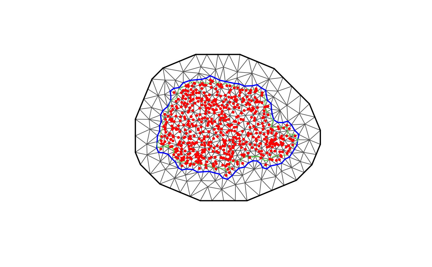

Setting up the data frame

In place of a inla.stack, we can set up a data.frame() to use inlabru. We refer the reader to vignettes in https://inlabru-org.github.io/inlabru/index.html for further details.

prdata <- data.frame(long = coords[,1], lat = coords[,2], 
                        seaDist = inla.group(seaDist), y = Y)
coordinates(prdata) <- c("long","lat")

Setting up the rSPDE model

To set up an rSPDEmodel, all we need is the mesh. By default it will assume that we want to estimate the smoothness parameter \(\nu\) and to do a covariance-based rational approximation of order 2.

Later in this vignette we will also see other options for setting up rSPDE models such as keeping the smoothness parameter fixed and/or increasing the order of the covariance-based rational approximation.

Therefore, to set up a model all we have to do is use the rspde.matern() function:

rspde_model <- rspde.matern(mesh = prmesh)

Notice that this function is very reminiscent of R-INLA’s inla.spde2.matern() function.

We will assume the following linkage between model components and observations \[\eta(s) \sim A x(s) + A \text{ Intercept} + \text{seaDist}.\] \(\eta(s)\) will then be used in the observation-likelihood, \[y_i\mid \eta(s_i),\theta \sim \Gamma(\exp(\eta (s_i)), c\phi).\]

Model fitting

We will build a model using the distance to the sea \(x_i\) as a covariate through an improper CAR(1) model with \(\beta_{ij}=1(i\sim j)\), which R-INLA calls a random walk of order 1. We will fit it in inlabru’s style:

cmp <- y ~ Intercept(1) + distSea(seaDist, model="rw1") +
field(coordinates, model = rspde_model)

To fit the model we simply use the bru() function:

rspde_fit <- bru(cmp, data = prdata,
  family = "Gamma",
  options = list(
    control.inla = list(int.strategy = "eb"),
    verbose = FALSE)
)

inlabru results

We can look at some summaries of the posterior distributions for the parameters, for example the fixed effects (i.e. the intercept) and the hyper-parameters (i.e. dispersion in the gamma likelihood, the precision of the RW1, and the parameters of the spatial field):

summary(rspde_fit)

## inlabru version: 2.10.1
## INLA version: 24.04.01
## Components:
## Intercept: main = linear(1), group = exchangeable(1L), replicate = iid(1L)
## distSea: main = rw1(seaDist), group = exchangeable(1L), replicate = iid(1L)
## field: main = cgeneric(coordinates), group = exchangeable(1L), replicate = iid(1L)
## Likelihoods:
##   Family: 'Gamma'
##     Data class: 'SpatialPointsDataFrame'
##     Predictor: y ~ .
## Time used:
##     Pre = 0.412, Running = 15.5, Post = 0.131, Total = 16.1 
## Fixed effects:
##            mean    sd 0.025quant 0.5quant 0.975quant  mode kld
## Intercept 1.943 0.048      1.849    1.943      2.037 1.943   0
## 
## Random effects:
##   Name     Model
##     distSea RW1 model
##    field CGeneric
## 
## Model hyperparameters:
##                                                    mean       sd 0.025quant
## Precision parameter for the Gamma observations   13.945    1.003     12.053
## Precision for distSea                          8019.268 4789.768   2268.116
## Theta1 for field                                 -0.194    1.087     -2.140
## Theta2 for field                                  1.073    0.478      0.087
## Theta3 for field                                 -1.793    0.832     -3.559
##                                                0.5quant 0.975quant     mode
## Precision parameter for the Gamma observations   13.917     16.000   13.876
## Precision for distSea                          6896.528  20381.349 5066.895
## Theta1 for field                                 -0.252      2.118   -0.534
## Theta2 for field                                  1.088      1.967    1.156
## Theta3 for field                                 -1.750     -0.299   -1.541
## 
## Deviance Information Criterion (DIC) ...............: 2486.61
## Deviance Information Criterion (DIC, saturated) ....: 714.17
## Effective number of parameters .....................: 100.31
## 
## Watanabe-Akaike information criterion (WAIC) ...: 2491.85
## Effective number of parameters .................: 91.51
## 
## Marginal log-Likelihood:  -1259.69 
##  is computed 
## Posterior summaries for the linear predictor and the fitted values are computed
## (Posterior marginals needs also 'control.compute=list(return.marginals.predictor=TRUE)')

Let \(\theta_1 = \textrm{Theta1}\), \(\theta_2=\textrm{Theta2}\) and \(\theta_3=\textrm{Theta3}\). In terms of the SPDE \[(\kappa^2 I - \Delta)^{\alpha/2}(\tau u) = \mathcal{W},\] where \(\alpha = \nu + d/2\), we have that \[\tau = \exp(\theta_1),\quad \kappa = \exp(\theta_2), \] and by default \[\nu = 4\Big(\frac{\exp(\theta_3)}{1+\exp(\theta_3)}\Big).\] The number 4 comes from the upper bound for \(\nu\), which is discussed in R-INLA implementation of the rational SPDE approach vignette.

In general, we have \[\nu = \nu_{UB}\Big(\frac{\exp(\theta_3)}{1+\exp(\theta_3)}\Big),\] where \(\nu_{UB}\) is the value of the upper bound for the smoothness parameter \(\nu\).

Another choice for prior for \(\nu\) is a truncated lognormal distribution and is also discussed in R-INLA implementation of the rational SPDE approach vignette.

inlabru results in the original scale

We can obtain outputs with respect to parameters in the original scale by using the function rspde.result():

result_fit <- rspde.result(rspde_fit, "field", 
                rspde_model)
summary(result_fit)

##           mean      sd 0.025quant 0.5quant 0.975quant     mode
## tau   1.563800 2.60857   0.119450 0.761565    8.12391 0.277172
## kappa 3.263400 1.55804   1.102340 2.981370    7.09768 2.418620
## nu    0.679649 0.41989   0.112659 0.599840    1.69199 0.354337

We can also plot the posterior densities. To this end we will use the gg_df() function, which creates ggplot2 user-friendly data frames:

posterior_df_fit <- gg_df(result_fit)

ggplot(posterior_df_fit) + geom_line(aes(x = x, y = y)) + 
facet_wrap(~parameter, scales = "free") + labs(y = "Density")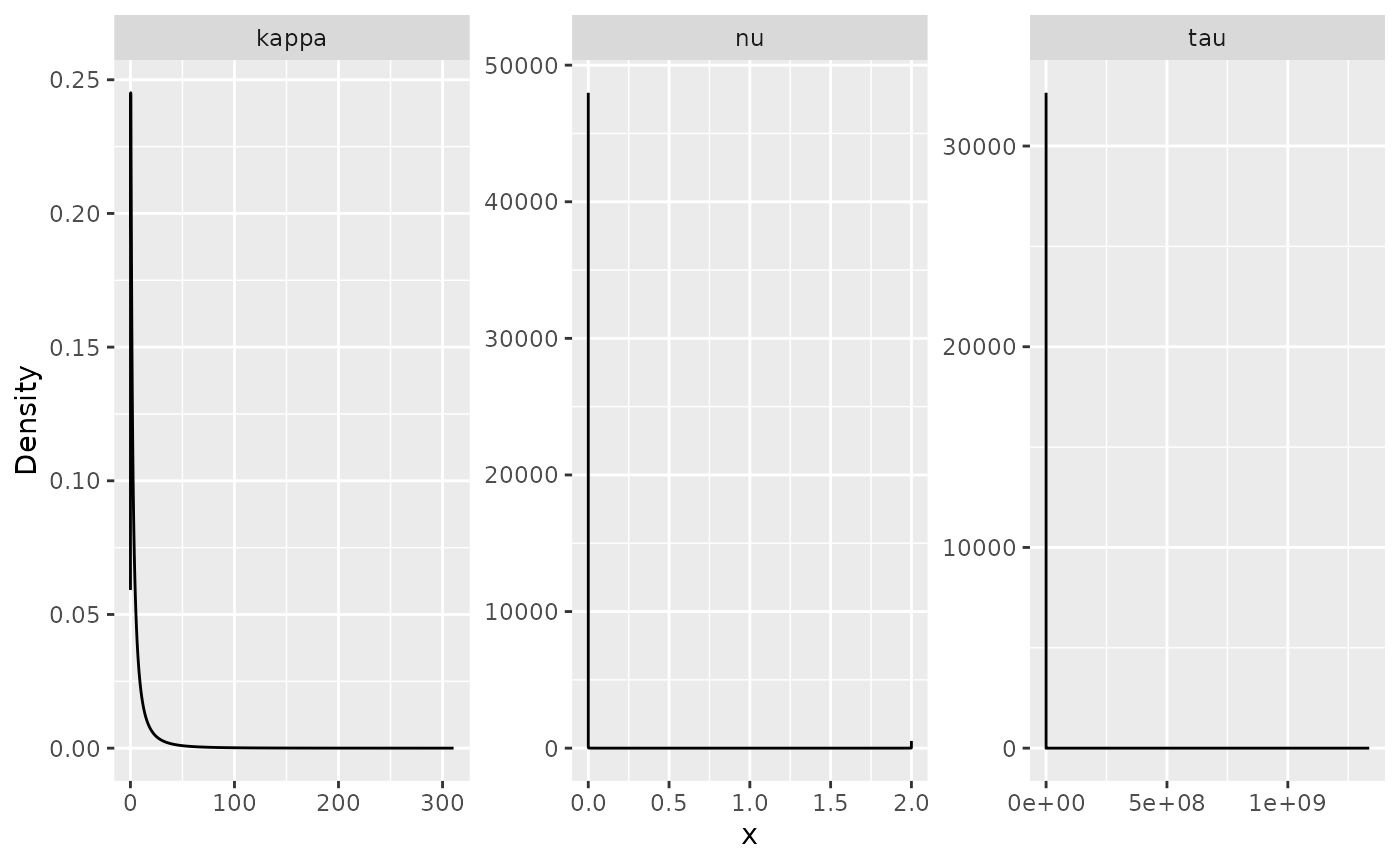

We can also obtain the summary on a different parameterization by setting the parameterization argument on the rspde.result() function:

result_fit_matern <- rspde.result(rspde_fit, "field", 
                rspde_model, parameterization = "matern")
summary(result_fit_matern)

##             mean        sd 0.025quant 0.5quant 0.975quant     mode
## std.dev 0.222062 0.0880472  0.0404516 0.237899   0.365007 0.269044
## range   0.766752 0.2810510  0.3459280 0.724403   1.427580 0.639382
## nu      0.679649 0.4198900  0.1126590 0.599840   1.691990 0.354337

In a similar manner, we can obtain posterior plots on the matern parameterization:

posterior_df_fit_matern <- gg_df(result_fit_matern)

ggplot(posterior_df_fit_matern) + geom_line(aes(x = x, y = y)) + 
facet_wrap(~parameter, scales = "free") + labs(y = "Density")

Predictions

Let us now obtain predictions (i.e. do kriging) of the expected precipitation on a dense grid in the region.

We begin by creating the grid in which we want to do the predictions. To this end, we can use the fm_evaluator() function:

nxy <- c(150, 100)
projgrid <- fm_evaluator(prmesh,
  xlim = range(PRborder[, 1]),
  ylim = range(PRborder[, 2]), dims = nxy
)

This lattice contains 150 × 100 locations. One can easily change the resolution of the kriging prediction by changing nxy. Let us find the cells that are outside the region of interest so that we do not plot the estimates there.

xy.in <- inout(projgrid$lattice$loc, cbind(PRborder[, 1], PRborder[, 2]))

Let us plot the locations that we will do prediction:

coord.prd <- projgrid$lattice$loc[xy.in, ]
plot(coord.prd, type = "p", cex = 0.1)
lines(PRborder)
points(coords[, 1], coords[, 2], pch = 19, cex = 0.5, col = "red")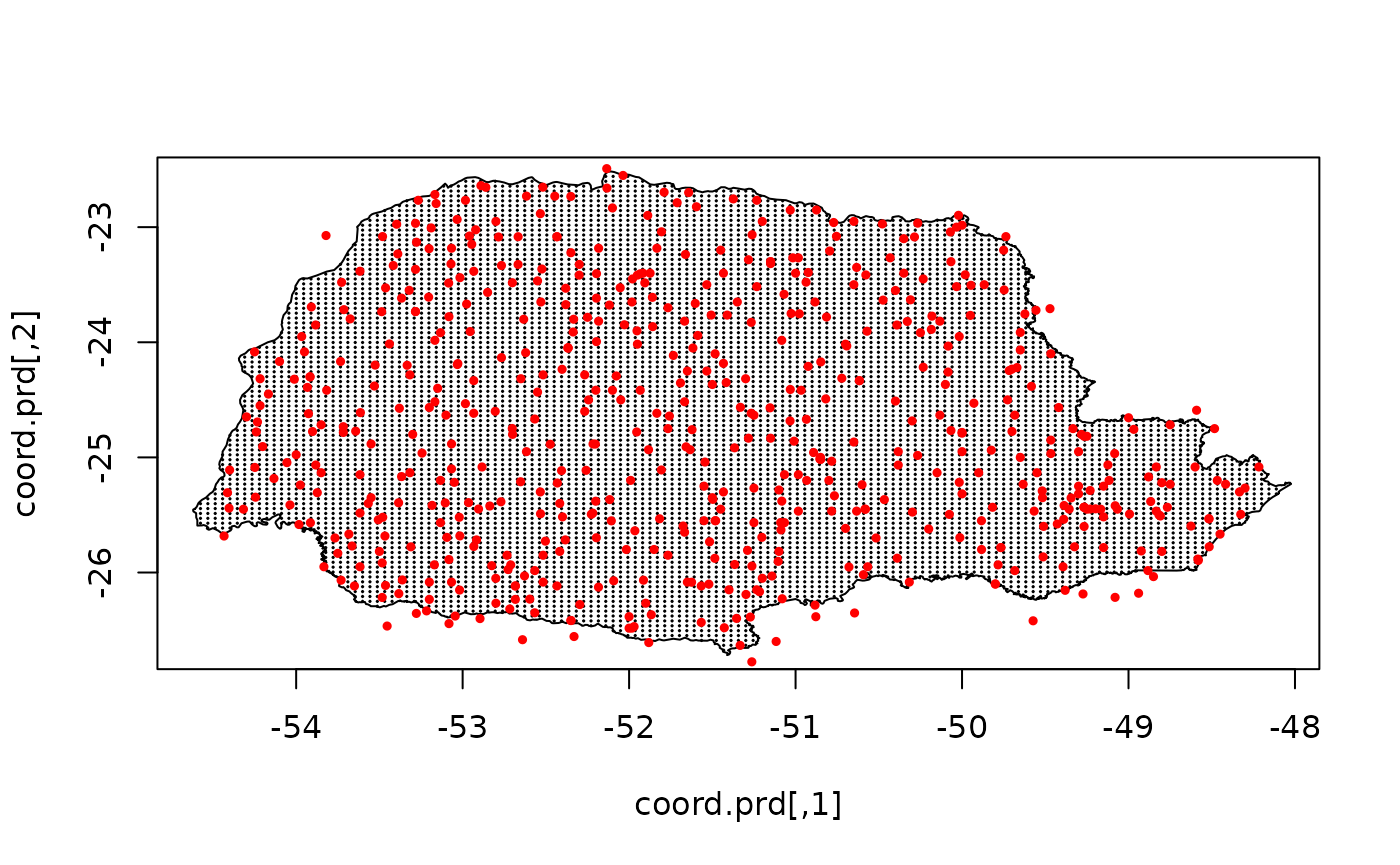

Let us now create a data.frame() of the coordinates:

coord.prd.df <- data.frame(x1 = coord.prd[,1],
                            x2 = coord.prd[,2])
coordinates(coord.prd.df) <- c("x1", "x2")

Since we are using distance to the sea as a covariate, we also have to calculate this covariate for the prediction locations. Finally, we add the prediction location to our prediction data.frame(), namely, coord.prd.df:

seaDist.prd <- apply(spDists(coord.prd,
  PRborder[1034:1078, ],
  longlat = TRUE
), 1, min)
coord.prd.df$seaDist <- seaDist.prd

pred_obs <- predict(rspde_fit, coord.prd.df, 
        ~exp(Intercept + field + distSea))

Let us now build the data frame with the results:

pred_df <- pred_obs@data
pred_df <- cbind(pred_df, pred_obs@coords)

Finally, we plot the results. First the predicted mean:

ggplot(pred_df, aes(x = x1, y = x2, fill = mean)) +
  geom_raster() +
  scale_fill_viridis()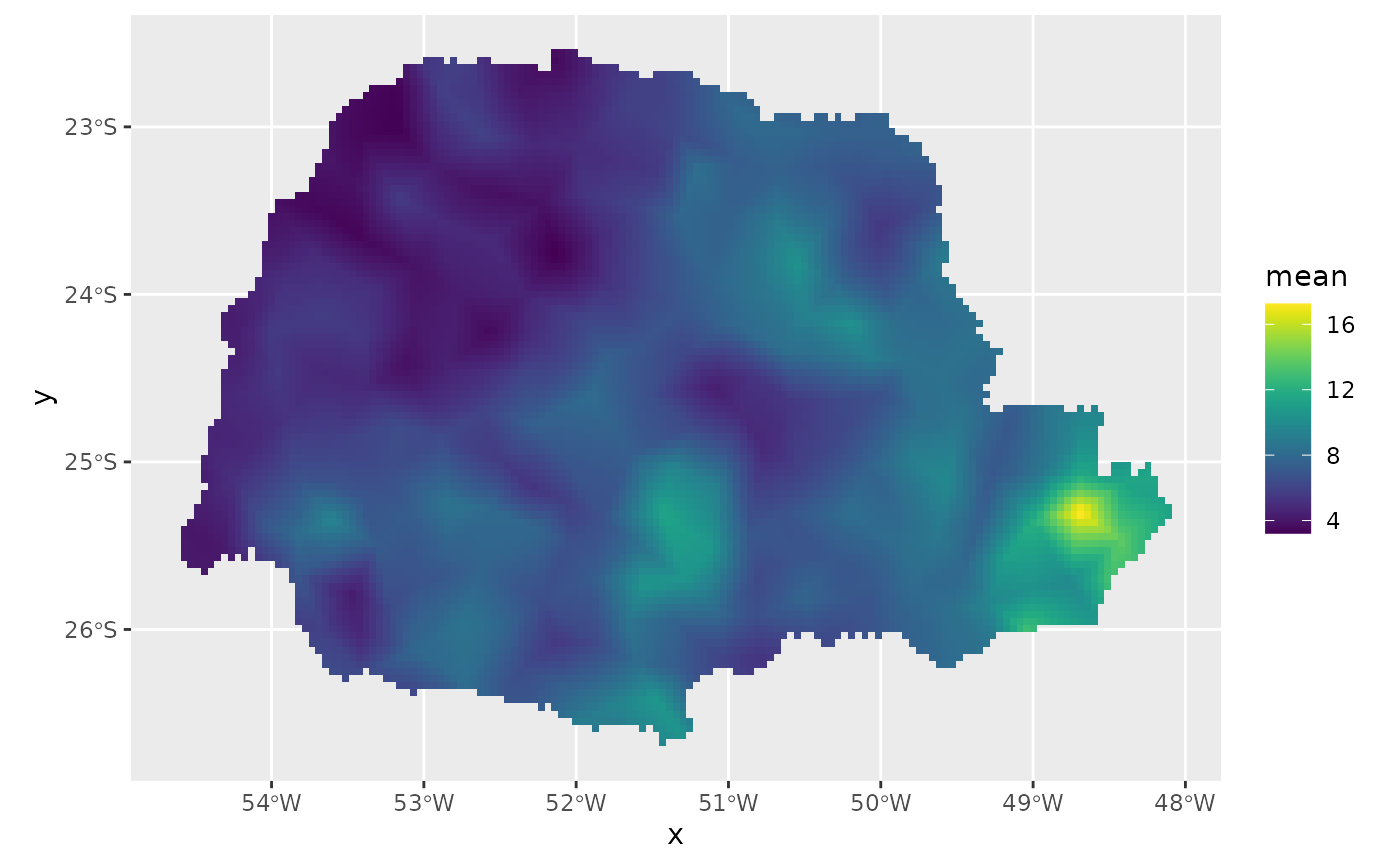

Then, the std. deviations:

ggplot(pred_df, aes(x = x1, y = x2, fill = sd)) +
  geom_raster() + scale_fill_viridis()

An example with replicates

For this example we will simulate a data with replicates. We will use the same example considered in the Rational approximation with the rSPDE package vignette (the only difference is the way the data is organized). We also refer the reader to this vignette for a description of the function matern.operators(), along with its methods (for instance, the simulate() method).

Simulating the data

Let us consider a simple Gaussian linear model with 30 independent replicates of a latent spatial field \(x(\mathbf{s})\), observed at the same \(m\) locations, \(\{\mathbf{s}_1 , \ldots , \mathbf{s}_m \}\), for each replicate. For each \(i = 1,\ldots,m,\) we have

\[\begin{align} y_i &= x_1(\mathbf{s}_i)+\varepsilon_i,\\ \vdots &= \vdots\\ y_{i+29m} &= x_{30}(\mathbf{s}_i) + \varepsilon_{i+29m}, \end{align}\]

where \(\varepsilon_1,\ldots,\varepsilon_{30m}\) are iid normally distributed with mean 0 and standard deviation 0.1.

We use the basis function representation of \(x(\cdot)\) to define the \(A\) matrix linking the point locations to the mesh. We also need to account for the fact that we have 30 replicates at the same locations. To this end, the \(A\) matrix we need can be generated by spde.make.A() function. The reason being that we are sampling \(x(\cdot)\) directly and not the latent vector described in the introduction of the Rational approximation with the rSPDE package vignette.

We begin by creating the mesh:

m <- 200
loc_2d_mesh <- matrix(runif(m * 2), m, 2)
mesh_2d <- fm_mesh_2d(
  loc = loc_2d_mesh,
  cutoff = 0.05,
  offset = c(0.1, 0.4),
  max.edge = c(0.05, 0.5)
)
plot(mesh_2d, main = "")
points(loc_2d_mesh[, 1], loc_2d_mesh[, 2])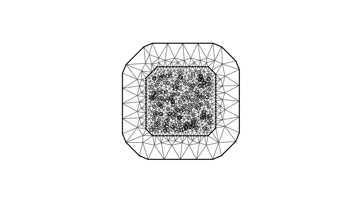

We then compute the \(A\) matrix, which is needed for simulation, and connects the observation locations to the mesh. To this end we will use the spde.make.A() helper function, which is a wrapper that uses the functions fm_basis(), fm_block() and fm_row_kron() from the fmesher package.

n.rep <- 30
A <- spde.make.A(
  mesh = mesh_2d,
  loc = loc_2d_mesh,
  index = rep(1:m, times = n.rep),
  repl = rep(1:n.rep, each = m)
)

Notice that for the simulated data, we should use the \(A\) matrix from spde.make.A() function instead of the rspde.make.A().

We will now simulate a latent process with standard deviation \(\sigma=1\) and range \(0.1\). We will use \(\nu=0.5\) so that the model has an exponential covariance function. To this end we create a model object with the matern.operators() function:

nu <- 0.5
sigma <- 1
range <- 0.1
kappa <- sqrt(8 * nu) / range
tau <- sqrt(gamma(nu) / (sigma^2 * kappa^(2 * nu) * (4 * pi) * gamma(nu + 1)))
d <- 2
operator_information <- matern.operators(
  mesh = mesh_2d,
  nu = nu,
  range = range,
  sigma = sigma,
  m = 2,
  parameterization = "matern"
)

More details on this function can be found at the Rational approximation with the rSPDE package vignette.

To simulate the latent process all we need to do is to use the simulate() method on the operator_information object. We then obtain the simulated data \(y\) by connecting with the \(A\) matrix and adding the gaussian noise.

set.seed(1)
u <- simulate(operator_information, nsim = n.rep)
y <- as.vector(A %*% as.vector(u)) +
  rnorm(m * n.rep) * 0.1

The first replicate of the simulated random field as well as the observation locations are shown in the following figure.

proj <- fm_evaluator(mesh_2d, dims = c(100, 100))

df_field <- data.frame(x = proj$lattice$loc[,1],
                        y = proj$lattice$loc[,2],
                        field = as.vector(fm_evaluate(proj, 
                        field = as.vector(u[, 1]))),
                        type = "field")

df_loc <- data.frame(x = loc_2d_mesh[, 1],
                      y = loc_2d_mesh[, 2],
                      field = y[1:m],
                      type = "locations")
df_plot <- rbind(df_field, df_loc)

ggplot(df_plot) + aes(x = x, y = y, fill = field) +
        facet_wrap(~type) + xlim(0,1) + ylim(0,1) + 
        geom_raster(data = df_field) +
        geom_point(data = df_loc, aes(colour = field),
        show.legend = FALSE) + 
        scale_fill_viridis() + scale_colour_viridis()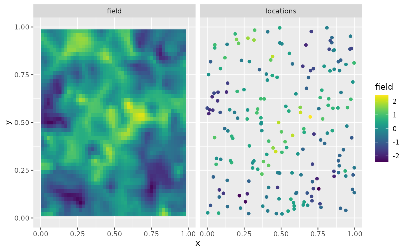

Fitting the inlabru rSPDE model

Let us then use the rational SPDE approach to fit the data.

We begin by creating the model object.

rspde_model.rep <- rspde.matern(mesh = mesh_2d,
          parameterization = "spde")

Let us now create the data.frame() and the vector with the replicates indexes:

rep.df <- data.frame(y = y, x1 = rep(loc_2d_mesh[,1], n.rep),
                      x2 = rep(loc_2d_mesh[,2], n.rep))
coordinates(rep.df) <- c("x1", "x2")
repl <- rep(1:n.rep, each=m)

Let us create the component and fit. It is extremely important not to forget the replicate when fitting model with the bru() function. It will not produce warning and might fit some meaningless model.

cmp.rep <-
  y ~ -1 + field(coordinates,
    model = rspde_model.rep,
    replicate = repl
  )


rspde_fit.rep <-
  bru(cmp.rep,
    data = rep.df,
    family = "gaussian"
  )

We can get the summary:

summary(rspde_fit.rep)

## inlabru version: 2.10.1
## INLA version: 24.04.01
## Components:
## field: main = cgeneric(coordinates), group = exchangeable(1L), replicate = iid(repl)
## Likelihoods:
##   Family: 'gaussian'
##     Data class: 'SpatialPointsDataFrame'
##     Predictor: y ~ .
## Time used:
##     Pre = 0.234, Running = 139, Post = 9.13, Total = 148 
## Random effects:
##   Name     Model
##     field CGeneric
## 
## Model hyperparameters:
##                                          mean    sd 0.025quant 0.5quant
## Precision for the Gaussian observations 92.89 4.670      83.81    92.85
## Theta1 for field                        -2.82 0.230      -3.26    -2.82
## Theta2 for field                         3.09 0.052       2.98     3.09
## Theta3 for field                        -1.74 0.112      -1.97    -1.74
##                                         0.975quant  mode
## Precision for the Gaussian observations     102.19 92.94
## Theta1 for field                             -2.36 -2.84
## Theta2 for field                              3.19  3.09
## Theta3 for field                             -1.53 -1.73
## 
## Deviance Information Criterion (DIC) ...............: -5257.71
## Deviance Information Criterion (DIC, saturated) ....: 10907.68
## Effective number of parameters .....................: 4902.87
## 
## Watanabe-Akaike information criterion (WAIC) ...: -6369.35
## Effective number of parameters .................: 2773.29
## 
## Marginal log-Likelihood:  -4776.95 
##  is computed 
## Posterior summaries for the linear predictor and the fitted values are computed
## (Posterior marginals needs also 'control.compute=list(return.marginals.predictor=TRUE)')

and the summary in the user’s scale:

result_fit_rep <- rspde.result(rspde_fit.rep, "field", rspde_model.rep)
summary(result_fit_rep)

##             mean       sd 0.025quant   0.5quant 0.975quant       mode
## tau    0.0611462 0.014275  0.0384862  0.0592769  0.0942941  0.0555488
## kappa 21.9520000 1.129600 19.7868000 21.9363000 24.2205000 21.9207000
## nu     0.5985140 0.056273  0.4916910  0.5975060  0.7123410  0.5967940

result_df <- data.frame(
  parameter = c("tau", "kappa", "nu"),
  true = c(tau, kappa, nu),
  mean = c(
    result_fit_rep$summary.tau$mean,
    result_fit_rep$summary.kappa$mean,
    result_fit_rep$summary.nu$mean
  ),
  mode = c(
    result_fit_rep$summary.tau$mode,
    result_fit_rep$summary.kappa$mode,
    result_fit_rep$summary.nu$mode
  )
)
print(result_df)

##   parameter        true        mean        mode
## 1       tau  0.08920621  0.06114624  0.05554878
## 2     kappa 20.00000000 21.95200688 21.92073204
## 3        nu  0.50000000  0.59851360  0.59679419

Let us also obtain the summary on the matern parameterization:

result_fit_rep_matern <- rspde.result(rspde_fit.rep, "field", rspde_model.rep, 
                          parameterization = "matern")
summary(result_fit_rep_matern)

##              mean         sd 0.025quant  0.5quant 0.975quant      mode
## std.dev 1.0492400 0.03589170  0.9572360 1.0576200   1.097540 1.0681800
## range   0.0997823 0.00418084  0.0918119 0.0996863   0.108367 0.0995195
## nu      0.5985140 0.05627300  0.4916910 0.5975060   0.712341 0.5967940

result_df_matern <- data.frame(
  parameter = c("std_dev", "range", "nu"),
  true = c(sigma, range, nu),
  mean = c(
    result_fit_rep_matern$summary.std.dev$mean,
    result_fit_rep_matern$summary.range$mean,
    result_fit_rep_matern$summary.nu$mean
  ),
  mode = c(
    result_fit_rep$summary.std.dev$mode,
    result_fit_rep$summary.range$mode,
    result_fit_rep$summary.nu$mode
  )
)
print(result_df_matern)

##   parameter true       mean      mode
## 1   std_dev  1.0 1.04923571 0.5967942
## 2     range  0.1 0.09978233 0.5967942
## 3        nu  0.5 0.59851360 0.5967942

An example with a non-stationary model

Our goal now is to show how one can fit model with non-stationary \(\sigma\) (std. deviation) and non-stationary \(\rho\) (a range parameter). One can also use the parameterization in terms of non-stationary SPDE parameters \(\kappa\) and \(\tau\).

For this example we will consider simulated data.

Simulating the data

Let us consider a simple Gaussian linear model with a latent spatial field \(x(\mathbf{s})\), defined on the rectangle \((0,10) \times (0,5)\), where the std. deviation and range parameter satisfy the following log-linear regressions: \[\begin{align} \log(\sigma(\mathbf{s})) &= \theta_1 + \theta_3 b(\mathbf{s}),\\ \log(\rho(\mathbf{s})) &= \theta_2 + \theta_3 b(\mathbf{s}), \end{align}\] where \(b(\mathbf{s}) = (s_1-5)/10\). We assume the data is observed at \(m\) locations, \(\{\mathbf{s}_1 , \ldots , \mathbf{s}_m \}\). For each \(i = 1,\ldots,m,\) we have

\[y_i = x_1(\mathbf{s}_i)+\varepsilon_i,\]

where \(\varepsilon_1,\ldots,\varepsilon_{m}\) are iid normally distributed with mean 0 and standard deviation 0.1.

We begin by defining the domain and creating the mesh:

rec_domain <- cbind(c(0, 1, 1, 0, 0) * 10, c(0, 0, 1, 1, 0) * 5)

mesh <- fm_mesh_2d(loc.domain = rec_domain, cutoff = 0.1, 
  max.edge = c(0.5, 1.5), offset = c(0.5, 1.5))

We follow the same structure as INLA. However, INLA only allows one to specify B.tau and B.kappa matrices, and, in INLA, if one wants to parameterize in terms of range and standard deviation one needs to do it manually. Here we provide the option to directly provide the matrices B.sigma and B.range.

The usage of the matrices B.tau and B.kappa are identical to the corresponding ones in inla.spde2.matern() function. The matrices B.sigma and B.range work in the same way, but they parameterize the stardard deviation and range, respectively.

The columns of the B matrices correspond to the same parameter. The first column does not have any parameter to be estimated, it is a constant column.

So, for instance, if one wants to share a parameter with both sigma and range (or with both tau and kappa), one simply let the corresponding column to be nonzero on both B.sigma and B.range (or on B.tau and B.kappa).

We will assume \(\nu = 0.8\), \(\theta_1 = 0, \theta_2 = 1\) and \(\theta_3=1\). Let us now build the model to obtain the sample with the spde.matern.operators() function:

nu <- 0.8
true_theta <- c(0,1, 1)
B.sigma = cbind(0, 1, 0, (mesh$loc[,1] - 5) / 10)
B.range = cbind(0, 0, 1, (mesh$loc[,1] - 5) / 10)

# SPDE model
op_cov_ns <- spde.matern.operators(mesh = mesh, 
  theta = true_theta,
  nu = nu,
  B.sigma = B.sigma, 
  B.range = B.range, m = 2,
  parameterization = "matern")

Let us now sample the data with the simulate() method:

u <- as.vector(simulate(op_cov_ns, seed = 123))

Let us now obtain 600 random locations on the rectangle and compute the \(A\) matrix:

m <- 600
loc_mesh <- cbind(runif(m) * 10, runif(m) * 5)

A <- spde.make.A(
  mesh = mesh,
  loc = loc_mesh
)

We can now generate the response vector y:

y <- as.vector(A %*% as.vector(u)) + rnorm(m) * 0.1

Fitting the inlabru rSPDE model

Let us then use the rational SPDE approach to fit the data.

We begin by creating the model object. We are creating a new one so that we do not start the estimation at the true values.

rspde_model_nonstat <- rspde.matern(mesh = mesh,
  B.sigma = B.sigma,
  B.range = B.range,
  parameterization = "matern")

Let us now create the data.frame() and the vector with the replicates indexes:

nonstat_df <- data.frame(y = y, x1 = loc_mesh[,1],
                      x2 = loc_mesh[,2])
coordinates(nonstat_df) <- c("x1", "x2")

cmp_nonstat <-
  y ~ -1 + field(coordinates,
    model = rspde_model_nonstat
  )


rspde_fit_nonstat <-
  bru(cmp_nonstat,
    data = nonstat_df,
    family = "gaussian",
    options = list(verbose = FALSE)
  )

We can get the summary:

summary(rspde_fit_nonstat)

## inlabru version: 2.10.1
## INLA version: 24.04.01
## Components:
## field: main = cgeneric(coordinates), group = exchangeable(1L), replicate = iid(1L)
## Likelihoods:
##   Family: 'gaussian'
##     Data class: 'SpatialPointsDataFrame'
##     Predictor: y ~ .
## Time used:
##     Pre = 0.188, Running = 108, Post = 0.334, Total = 109 
## Random effects:
##   Name     Model
##     field CGeneric
## 
## Model hyperparameters:
##                                            mean     sd 0.025quant 0.5quant
## Precision for the Gaussian observations 104.865 10.860     84.999  104.347
## Theta1 for field                         -0.121  0.109     -0.336   -0.121
## Theta2 for field                          0.762  0.186      0.386    0.766
## Theta3 for field                          1.123  0.232      0.647    1.130
## Theta4 for field                         -1.177  0.173     -1.511   -1.180
##                                         0.975quant   mode
## Precision for the Gaussian observations    127.707 103.40
## Theta1 for field                             0.093  -0.12
## Theta2 for field                             1.120   0.78
## Theta3 for field                             1.558   1.16
## Theta4 for field                            -0.829  -1.19
## 
## Deviance Information Criterion (DIC) ...............: -738.00
## Deviance Information Criterion (DIC, saturated) ....: 946.46
## Effective number of parameters .....................: 344.26
## 
## Watanabe-Akaike information criterion (WAIC) ...: -769.98
## Effective number of parameters .................: 236.05
## 
## Marginal log-Likelihood:  -14.35 
##  is computed 
## Posterior summaries for the linear predictor and the fitted values are computed
## (Posterior marginals needs also 'control.compute=list(return.marginals.predictor=TRUE)')

We can obtain outputs with respect to parameters in the original scale by using the function rspde.result():

result_fit_nonstat <- rspde.result(rspde_fit_nonstat, "field", rspde_model_nonstat)
summary(result_fit_nonstat)

##                    mean       sd 0.025quant  0.5quant 0.975quant      mode
## Theta1.matern -0.120880 0.109110  -0.336195 -0.120704  0.0934105 -0.119974
## Theta2.matern  0.762460 0.186413   0.385976  0.765675  1.1197900  0.779599
## Theta3.matern  1.123380 0.231573   0.646829  1.130390  1.5575100  1.162020
## nu             0.947814 0.124464   0.724777  0.940134  1.2123700  0.922393

Let us compare the mean to the true values of the parameters:

summ_res_nonstat <- summary(result_fit_nonstat)
result_df <- data.frame(
  parameter = result_fit_nonstat$params,
  true = c(true_theta, nu),
  mean = summ_res_nonstat[,1],
  mode = summ_res_nonstat[,6]
)
print(result_df)

##       parameter true      mean      mode
## 1 Theta1.matern  0.0 -0.120880 -0.119974
## 2 Theta2.matern  1.0  0.762460  0.779599
## 3 Theta3.matern  1.0  1.123380  1.162020
## 4            nu  0.8  0.947814  0.922393

We can also plot the posterior densities. To this end we will use the gg_df() function, which creates ggplot2 user-friendly data frames:

posterior_df_fit <- gg_df(result_fit_nonstat)

ggplot(posterior_df_fit) + geom_line(aes(x = x, y = y)) + 
facet_wrap(~parameter, scales = "free") + labs(y = "Density")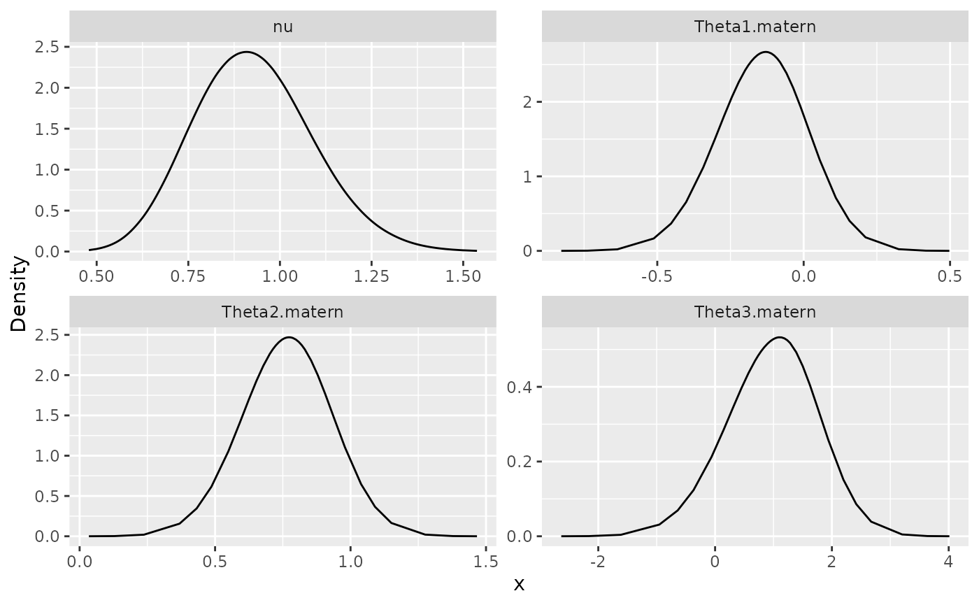

Comparing the results by cross-validation

We can compare the models fitted by inlabru by using the function cross_validation(). To illustrate, we will consider the nonstationary model rspde_fit_nonstat fitted in the previous example and a stationary fit of the same dataset.

Let us, then, fit a stationary model with the previous dataset. We start by defining the stationary model:

rspde_model_stat <- rspde.matern(mesh = mesh)

Then, inlabru’s component:

cmp_stat <-
  y ~ -1 + field(coordinates,
    model = rspde_model_stat
  )

We can now fit the model:

rspde_fit_stat <-
  bru(cmp_stat,
    data = nonstat_df,
    family = "gaussian",
    options = list(verbose = FALSE)
  )

To perform cross-validation, we create a list with the fitted models, and we pass this list to the cross_validation() function. It is also important to create a named list, so that the output has meaningful names for the models. We will perform a leave percentage out cross-validation, with the default that fits the model on 20% of the data, to predict 80% of the data.

Let us create the models list:

models <- list(stationary = rspde_fit_stat, 
                nonstationary = rspde_fit_nonstat)

We will now run the cross-validation on the models above. We set the cv_type to lpo to perform the leave percentage out cross-validation, there are also the k-fold (default) and loo options to perform k-fold and leave one out cross-validations, respectively. Observe that by default we are performing a pseudo cross-validation, that is, we will not refit the model for each fold, however only the training data will be used to perform the prediction.

cv_result <- cross_validation(models, cv_type = "lpo", print = FALSE)

We can now look at the results by printing cv_result. Observe that the best model with respect to each score is displayed in the last row.

cv_result

##           Model               dss               mse               crps
## 1    stationary -1.28754077084693 0.134149859404844 -0.192972600313429
## 2 nonstationary -1.30256889269139 0.132504006899066  -0.19212874417702
##            Best     nonstationary     nonstationary         stationary
##               scrps
## 1 0.486581799755334
## 2 0.484048783653525
##       nonstationary

The cross_validation() function also has the following useful options:

return_score_folds option, so that the scores for each fold can be returned in order to create confidence regions for the scores.
return_train_test To return the train and test indexes that were used to perform the cross-validation.
true_CV To perform true cross-validation, that is, the data will be fit again for each fold, which is more costly.
train_test_indexes In which the user can provide the indexes for the train and test sets.

More details can be found in the manual page of the cross_validation() function.

Further options of the `inlabru` implementation

There are several additional options that are available. For instance, it is possible to change the order of the rational approximation, the upper bound for the smoothness parameter (which may speed up the fit), change the priors, change the type of the rational approximation, among others. These options are described in the “Further options of the rSPDE-INLA implementation” section of the R-INLA implementation of the rational SPDE approach vignette. Observe that all these options are passed to the model through the rspde.matern() function, and therefore the resulting model object can directly be used in the bru() function, in an identical manner to the examples above.

References

Bolin, David, Alexandre B. Simas, and Zhen Xiong. 2023. “Covariance-Based Rational Approximations of Fractional SPDEs for Computationally Efficient Bayesian Inference.” Journal of Computational and Graphical Statistics.

Lindgren, Finn, Håvard Rue, and Johan Lindström. 2011. “An Explicit Link Between Gaussian Fields and Gaussian Markov Random Fields: The Stochastic Partial Differential Equation Approach.” Journal of the Royal Statistical Society. Series B. Statistical Methodology 73 (4): 423–98.

David Bolin and Alexandre B. Simas

Created: 2022-09-13. Last modified: 2024-04-01.

Introduction

An example with real data

An rSPDE model for precipitation

Examining the data

Creating the rSPDE model

Mesh

Setting up the data frame

Setting up the rSPDE model

Model fitting

inlabru results

inlabru results in the original scale

Predictions

An example with replicates

Simulating the data

Fitting the inlabru rSPDE model

An example with a non-stationary model

Simulating the data

Fitting the inlabru rSPDE model

Comparing the results by cross-validation

Further options of the `inlabru` implementation

References

inlabru implementation of the rational SPDE approach

David Bolin and Alexandre B. Simas

Created: 2022-09-13. Last modified: 2024-04-01.

Introduction

An example with real data

An rSPDE model for precipitation

Examining the data

Creating the rSPDE model

Mesh

Setting up the data frame

Setting up the rSPDE model

Model fitting

inlabru results

inlabru results in the original scale

Predictions

An example with replicates

Simulating the data

Fitting the inlabru rSPDE model

An example with a non-stationary model

Simulating the data

Fitting the inlabru rSPDE model

Comparing the results by cross-validation

Further options of the inlabru implementation

References

Further options of the `inlabru` implementation