R-INLA implementation of the rational SPDE approach

David Bolin and Alexandre B. Simas

Created: 2021-10-30. Last modified: 2024-07-25.

Introduction

In this vignette we will present the R-INLA implementation of the rational SPDE approach. For theoretical details we refer the reader to the Rational approximation with the rSPDE package vignette and to Bolin, Simas, and Xiong (2023).

We begin by providing a step-by-step illustration on how to use our implementation. To this end we will consider a real world data set that consists of precipitation measurements from the Paraná region in Brazil.

After the initial model fitting, we will show how to change some parameters of the model. In the end, we will also provide an example in which we have replicates.

It is important to mention that one can improve the performance by using the PARDISO solver. Please, go to https://www.pardiso-project.org/r-inla/#license to apply for a license. Also, use inla.pardiso() for instructions on how to enable the PARDISO sparse library.

Example with real data

To illustrate our implementation of rSPDE in R-INLA we will consider a dataset available in R-INLA. This data has also been used to illustrate the SPDE approach, see for instance the book Advanced Spatial Modeling with Stochastic Partial Differential Equations Using R and INLA and also the vignette Spatial Statistics using R-INLA and Gaussian Markov random fields. See also Lindgren, Rue, and Lindström (2011) for theoretical details on the standard SPDE approach.

The data consist of precipitation measurements from the Paraná region in Brazil and were provided by the Brazilian National Water Agency. The data were collected at 616 gauge stations in Paraná state, south of Brazil, for each day in 2011.

An rSPDE model for precipitation

We will follow the vignette Spatial Statistics using R-INLA and Gaussian Markov random fields. As precipitation data are always positive, we will assume it is Gamma distributed. R-INLA uses the following parameterization of the Gamma distribution, $$\Gamma(\mu, \phi): \pi (y) = \frac{1}{\Gamma(\phi)} \left(\frac{\phi}{\mu}\right)^{\phi} y^{\phi - 1} \exp\left(-\frac{\phi y}{\mu}\right) .$$ In this parameterization, the distribution has expected value $E(x) = \mu$ and variance $V(x) = \mu^2/(\phi)$, where$1/\phi$ is a dispersion parameter.

In this example $\mu$ will be modeled using a stochastic model that includes both covariates and spatial structure, resulting in the latent Gaussian model for the precipitation measurements $$\begin{align} y_i\mid \mu(s_i), \theta &\sim \Gamma(\mu(s_i),c\phi)\\ \log (\mu(s)) &= \eta(s) = \sum_k f_k(c_k(s))+u(s)\\ \theta &\sim \pi(\theta) \end{align},$$

where $y_i$ denotes the measurement taken at location $s_i$, $c_k(s)$ are covariates, $u(s)$ is a mean-zero Gaussian Matérn field, and $\theta$ is a vector containing all parameters of the model, including smoothness of the field. That is, by using the rSPDE model we will also be able to estimate the smoothness of the latent field.

Examining the data

We will be using R-INLA. To install R-INLA go to R-INLA Project.

We begin by loading some libraries we need to get the data and build the plots.

library(ggplot2)
library(INLA)
library(splancs)
library(viridis)

Let us load the data and the border of the region

data(PRprec)
data(PRborder)

The data frame contains daily measurements at 616 stations for the year 2011, as well as coordinates and altitude information for the measurement stations. We will not analyze the full spatio-temporal data set, but instead look at the total precipitation in January, which we calculate as

Y <- rowMeans(PRprec[, 3 + 1:31])

In the next snippet of code, we extract the coordinates and altitudes and remove the locations with missing values.

ind <- !is.na(Y)
Y <- Y[ind]
coords <- as.matrix(PRprec[ind, 1:2])
alt <- PRprec$Altitude[ind]

Let us build plot the precipitation observations using ggplot:

ggplot() +
  geom_point(aes(
    x = coords[, 1], y = coords[, 2],
    colour = Y
  ), size = 2, alpha = 1) +
  geom_path(aes(x = PRborder[, 1], y = PRborder[, 2])) +
  geom_path(aes(x = PRborder[1034:1078, 1], y = PRborder[
    1034:1078,
    2
  ]), colour = "red") + 
  scale_color_viridis()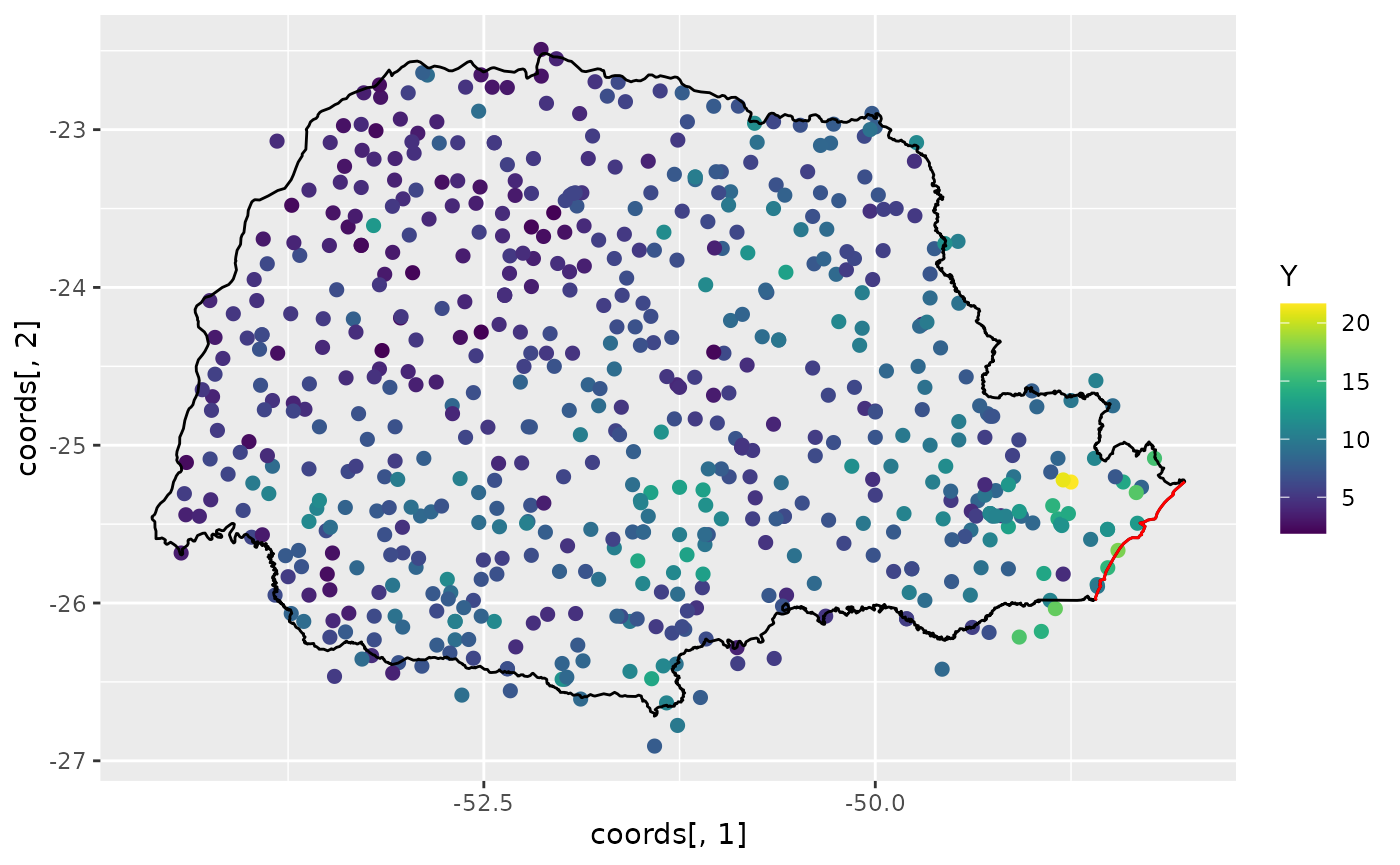

The red line in the figure shows the coast line, and we expect the distance to the coast to be a good covariate for precipitation. This covariate is not available, so let us calculate it for each observation location:

seaDist <- apply(spDists(coords, PRborder[1034:1078, ],
  longlat = TRUE
), 1, min)

Now, let us plot the precipitation as a function of the possible covariates:

par(mfrow = c(2, 2))
plot(coords[, 1], Y, cex = 0.5, xlab = "Longitude")
plot(coords[, 2], Y, cex = 0.5, xlab = "Latitude")
plot(seaDist, Y, cex = 0.5, xlab = "Distance to sea")
plot(alt, Y, cex = 0.5, xlab = "Altitude")

par(mfrow = c(1, 1))

Creating the rSPDE model

To use the R-INLA implementation of the rSPDE model we need to load the functions:

library(rSPDE)

The rSPDE-INLA implementation is very reminiscent of R-INLA, so its usage should be straightforward for R-INLA users. For instance, to create a rSPDE model, one would use rspde.matern() in place of inla.spde2.matern(). To create an index, one should use rspde.make.index() in place of inla.spde.make.index(). To create the A matrix, one should use rspde.make.A() in place of inla.spde.make.A(), and so on.

The main differences when comparing the arguments between the rSPDE-INLA implementation and the standard SPDE implementation in R-INLA, are the nu and rspde.order arguments, which are present in rSPDE-INLA implementation. We will see below how use these arguments.

Mesh

We can use fmesher for creating the mesh. We begin by loading the fmesher package:

library(fmesher)

Let us create a mesh which is based on a non-convex hull to avoid adding many small triangles outside the domain of interest:

prdomain <- fm_nonconvex_hull(coords, -0.03, -0.05, resolution = c(100, 100))
prmesh <- fm_mesh_2d(boundary = prdomain, max.edge = c(0.45, 1), cutoff = 0.2)

plot(prmesh, asp = 1, main = "")
lines(PRborder, col = 3)
points(coords[, 1], coords[, 2], pch = 19, cex = 0.5, col = "red")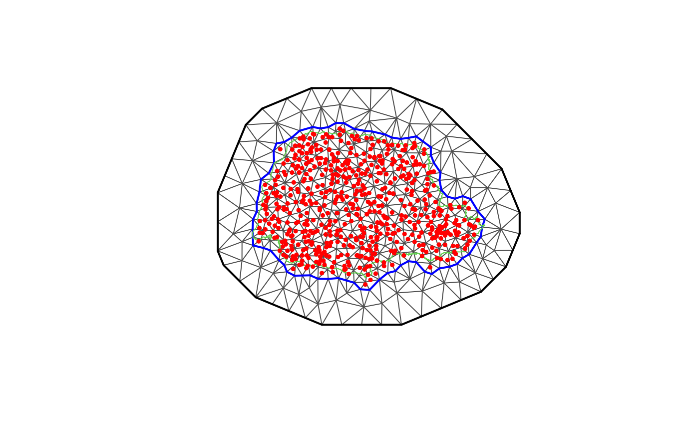

The observation matrix

We now create the $A$ matrix, that connects the mesh to the observation locations and then create the rSPDE model.

For this task, as we mentioned earlier, we need to use an rSPDEspecific function, whose name is very reminiscent to R-INLA’s standard SPDE approach, namely rspde.make.A() (in place of R-INLA’s inla.spde.make.A()). The reason for the need of this specific function is that the size of the $A$ matrix depends on the order of the rational approximation. The details can be found in the introduction of the Rational approximation with the rSPDE package vignette.

The default order is 2 for our covariance-based rational approximation. As mentioned in the introduction of the Rational approximation with the rSPDE package vignette, an approximation of order 2 in the covariance-based rational approximation has approximately the same computational cost as the operator-based rational approximation of order 1.

Recall that the latent process $u$ is a solution of $$(\kappa^2 I-\Delta)^{\alpha/2}(\tau u) = \mathcal{W},$$ where $\alpha = \nu + d/2$. We want to estimate all three parameters $\tau,\kappa$ and $\nu$, which is the default option of
the rSPDE-INLA implementation. However, there is also an option to fix the smoothness parameter $\nu$ to some predefined value and only estimate $\tau$ and $\kappa$. This will be discussed later.

In this first example we will assume we want a rational approximation of order 2. To this end we can use the rspde.make.A() function. Since we will assume order 2 and that we want to estimate smoothness, which are the default options in this function, the required parameters are simply the mesh and the locations:

Abar <- rspde.make.A(mesh = prmesh, loc = coords)

Setting up the rSPDE model

To set up an rSPDEmodel, all we need is the mesh. By default it will assume that we want to estimate the smoothness parameter $\nu$ and to do a covariance-based rational approximation of order 2.

Later in this vignette we will also see other options for setting up rSPDE models such as keeping the smoothness parameter fixed and/or increasing the order of the covariance-based rational approximation.

Therefore, to set up a model all we have to do is use the rspde.matern() function:

rspde_model <- rspde.matern(mesh = prmesh)

Note that this function is very reminiscent of R-INLA’s inla.spde2.matern() function. This is a pattern we have tried to keep consistent in the package: All the rSPDE versions of some R-INLA function will either replace inla or inla.spde or inla.spde2 by rspde.

The inla.stack

Since the covariates are already evaluated at the observation locations, we only want to apply the $A$ matrix to the spatial effect and not the fixed effects. We can use the inla.stack() function.

The difference, however, is that we need to use the function rspde.make.index() (in place of the standard inla.spde.make.index()) to create the index.

If one is using the default options, that is, to estimate the smoothness parameter $\nu$ and to do a rational approximation of order 2, the usage of rspde.make.index() is identical to the usage of inla.spde.make.index():

mesh.index <- rspde.make.index(name = "field", mesh = prmesh)

We can then create the stack in a standard manner:

stk.dat <- inla.stack(
  data = list(y = Y), A = list(Abar, 1), tag = "est",
  effects = list(
    c(
      mesh.index
    ),
    list(
      seaDist = inla.group(seaDist),
      Intercept = 1
    )
  )
)

Here the observation matrix $A$ is applied to the spatial effect and the intercept while an identity observation matrix, denoted by $1$, is applied to the covariates. This means the covariates are unaffected by the observation matrix.

The observation matrices in $A=list(Abar,1)$ are used to link the corresponding elements in the effects-list to the observations. Thus in our model the latent spatial field mesh.index and the intercept are linked to the log-expectation of the observations, i.e. $\eta(s)$, through the $A$-matrix. The covariates, on the other hand, are linked directly to $\eta(s)$. The stk.dat object defined above implies the following principal linkage between model components and observations $$\eta(s) \sim A x(s) + A \text{ Intercept} + \text{seaDist}.$$$\eta(s)$ will then be used in the observation-likelihood, $$y_i\mid \eta(s_i),\theta \sim \Gamma(\exp(\eta (s_i)), c\phi).$$

Model fitting

We will build a model using the distance to the sea $x_i$ as a covariate through an improper CAR(1) model with $\beta_{ij}=1(i\sim j)$, which R-INLA calls a random walk of order 1.

f.s <- y ~ -1 + Intercept + f(seaDist, model = "rw1") +
  f(field, model = rspde_model)

Here -1 is added to remove R’s implicit intercept, which is replaced by the explicit +Intercept from when we created the stack.

To fit the model we proceed as in the standard SPDE approach and we simply call inla().

rspde_fit <- inla(f.s,
  family = "Gamma", data = inla.stack.data(stk.dat),
  verbose = FALSE,
  control.inla = list(int.strategy = "eb"),
  control.predictor = list(A = inla.stack.A(stk.dat), compute = TRUE)
)

INLA results

We can look at some summaries of the posterior distributions for the parameters, for example the fixed effects (i.e. the intercept) and the hyper-parameters (i.e. dispersion in the gamma likelihood, the precision of the RW1, and the parameters of the spatial field):

summary(rspde_fit)

## Time used:
##     Pre = 0.548, Running = 25.4, Post = 0.211, Total = 26.1 
## Fixed effects:
##            mean    sd 0.025quant 0.5quant 0.975quant  mode kld
## Intercept 1.944 0.047      1.852    1.944      2.035 1.944   0
## 
## Random effects:
##   Name     Model
##     seaDist RW1 model
##    field CGeneric
## 
## Model hyperparameters:
##                                                    mean       sd 0.025quant
## Precision-parameter for the Gamma observations   13.917    1.015     12.094
## Precision for seaDist                          8288.218 5471.936   2341.554
## Theta1 for field                                  0.046    1.011     -1.752
## Theta2 for field                                  0.985    0.517     -0.092
## Theta3 for field                                 -2.013    0.866     -3.857
##                                                0.5quant 0.975quant     mode
## Precision-parameter for the Gamma observations   13.858     16.088   13.690
## Precision for seaDist                          6876.027  22754.620 4870.543
## Theta1 for field                                 -0.011      2.204   -0.289
## Theta2 for field                                  1.005      1.939    1.098
## Theta3 for field                                 -1.966     -0.465   -1.739
## 
## Marginal log-Likelihood:  -1259.43 
##  is computed 
## Posterior summaries for the linear predictor and the fitted values are computed
## (Posterior marginals needs also 'control.compute=list(return.marginals.predictor=TRUE)')

Let $\theta_1 = \textrm{Theta1}$, $\theta_2=\textrm{Theta2}$ and $\theta_3=\textrm{Theta3}$. In terms of the SPDE $$(\kappa^2 I - \Delta)^{\alpha/2}(\tau u) = \mathcal{W},$$ where $\alpha = \nu + d/2$, we have that $$\tau = \exp(\theta_1),\quad \kappa = \exp(\theta_2),$$ and by default $$\nu = 4\Big(\frac{\exp(\theta_3)}{1+\exp(\theta_3)}\Big).$$ The number 4 comes from the upper bound for $\nu$, which will be discussed later in this vignette.

In general, we have $$\nu = \nu_{UB}\Big(\frac{\exp(\theta_3)}{1+\exp(\theta_3)}\Big),$$ where $\nu_{UB}$ is the value of the upper bound for the smoothness parameter $\nu$.

Another choice for prior for $\nu$ is a truncated lognormal distribution and will also be discussed later in this vignette.

rSPDE-INLA results

We can obtain outputs with respect to parameters in the original scale by using the function rspde.result():

result_fit <- rspde.result(rspde_fit, "field", rspde_model)
summary(result_fit)

##           mean       sd 0.025quant 0.5quant 0.975quant     mode
## tau   1.822950 2.728870  0.1757630 0.969547    8.86728 0.400291
## kappa 3.041980 1.558550  0.9224710 2.749560    6.89875 2.131830
## nu    0.579906 0.384976  0.0843331 0.498132    1.53174 0.261022

To create plots of the posterior marginal densities, we can use the gg_df() function, which creates ggplot2-friendly data frames. The following figure shows the posterior marginal densities of the three parameters using the gg_df() function.

posterior_df_fit <- gg_df(result_fit)

ggplot(posterior_df_fit) + geom_line(aes(x = x, y = y)) + 
facet_wrap(~parameter, scales = "free") + labs(y = "Density")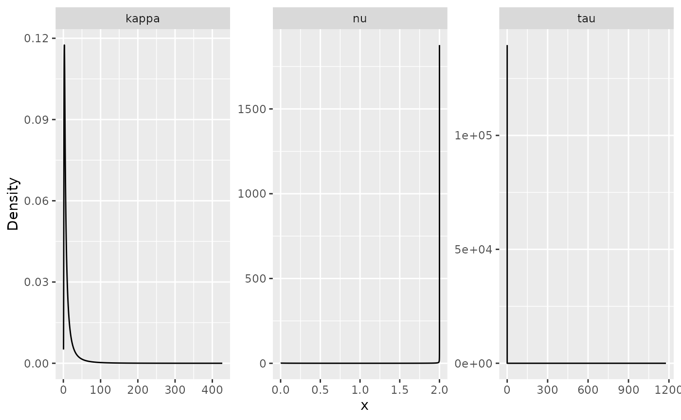

This function is reminiscent to the inla.spde.result() function with the main difference that it has the summary() and plot() methods implemented.

We can also obtain the results for the matern parameterization by setting the parameterization argument to matern:

result_fit_matern <- rspde.result(rspde_fit, "field", 
                      rspde_model, parameterization = "matern")
summary(result_fit_matern)

##             mean        sd 0.025quant 0.5quant 0.975quant     mode
## std.dev 0.215545 0.0831792  0.0448135 0.228992   0.353857 0.259930
## range   0.792596 0.3129550  0.3367000 0.737740   1.558960 0.657637
## nu      0.579906 0.3849760  0.0843331 0.498132   1.531740 0.261022

In a similar manner, we can obtain posterior plots on the matern parameterization:

posterior_df_fit_matern <- gg_df(result_fit_matern)

ggplot(posterior_df_fit_matern) + geom_line(aes(x = x, y = y)) + 
facet_wrap(~parameter, scales = "free") + labs(y = "Density")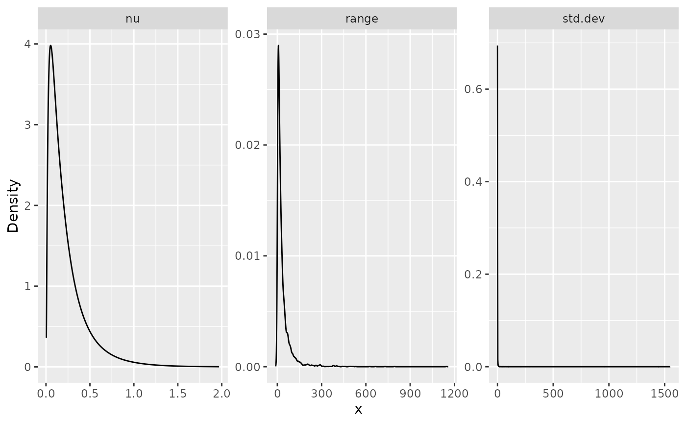

Predictions

Let us now obtain predictions (i.e. do kriging) of the expected precipitation on a dense grid in the region.

We begin by creating the grid in which we want to do the predictions. To this end, we can use the rspde.mesh.projector() function. This function has the same arguments as the function inla.mesh.projector(), with the only difference being that the rSPDE version also has an argument nu and an argument rspde.order. Thus, we proceed in the same fashion as we would in R-INLA’s standard SPDE implementation:

nxy <- c(150, 100)
projgrid <- rspde.mesh.projector(prmesh,
  xlim = range(PRborder[, 1]),
  ylim = range(PRborder[, 2]), dims = nxy
)

This lattice contains 150 × 100 locations. One can easily change the resolution of the kriging prediction by changing nxy. Let us find the cells that are outside the region of interest so that we do not plot the estimates there.

xy.in <- inout(projgrid$lattice$loc, cbind(PRborder[, 1], PRborder[, 2]))

Let us plot the locations that we will do prediction:

coord.prd <- projgrid$lattice$loc[xy.in, ]
plot(coord.prd, type = "p", cex = 0.1)
lines(PRborder)
points(coords[, 1], coords[, 2], pch = 19, cex = 0.5, col = "red")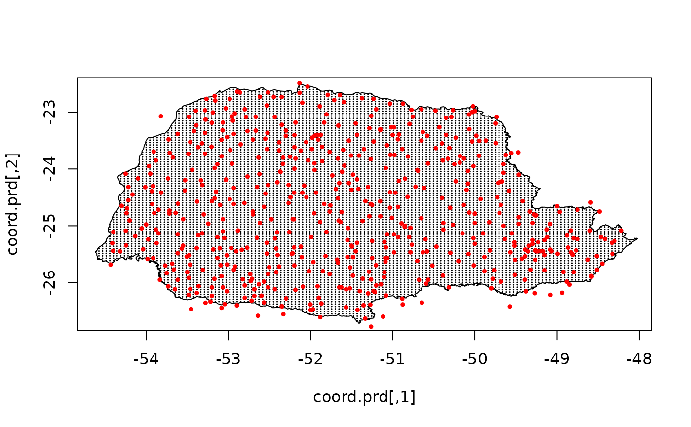

Now, there are a few ways we could calculate the kriging prediction. The simplest way is to evaluate the mean of all individual random effects in the linear predictor and then to calculate the exponential of their sum (since $\mu(s)=\exp(\eta(s))$ ). A more accurate way is to calculate the prediction jointly with the estimation, which unfortunately is quite computationally expensive if we do prediction on a fine grid. However, in this illustration, we proceed with this option to show how one can do it.

To this end, first, link the prediction coordinates to the mesh nodes through an $A$ matrix

A.prd <- projgrid$proj$A[xy.in, ]

Since we are using distance to the sea as a covariate, we also have to calculate this covariate for the prediction locations.

seaDist.prd <- apply(spDists(coord.prd,
  PRborder[1034:1078, ],
  longlat = TRUE
), 1, min)

We now make a stack for the prediction locations. We have no data at the prediction locations, so we set y= NA. We then join this stack with the estimation stack.

ef.prd <- list(
  c(mesh.index),
  list(
    long = inla.group(coord.prd[
      ,
      1
    ]), lat = inla.group(coord.prd[, 2]),
    seaDist = inla.group(seaDist.prd),
    Intercept = 1
  )
)
stk.prd <- inla.stack(
  data = list(y = NA),
  A = list(A.prd, 1), tag = "prd",
  effects = ef.prd
)
stk.all <- inla.stack(stk.dat, stk.prd)

Doing the joint estimation takes a while, and we therefore turn off the computation of certain things that we are not interested in, such as the marginals for the random effect. We will also use a simplified integration strategy (actually only using the posterior mode of the hyper-parameters) through the command control.inla = list(int.strategy = "eb"), i.e. empirical Bayes.

rspde_fitprd <- inla(f.s,
  family = "Gamma",
  data = inla.stack.data(stk.all),
  control.predictor = list(
    A = inla.stack.A(stk.all),
    compute = TRUE, link = 1
  ),
  control.compute = list(
    return.marginals = FALSE,
    return.marginals.predictor = FALSE
  ),
  control.inla = list(int.strategy = "eb")
)

We then extract the indices to the prediction nodes and then extract the mean and the standard deviation of the response:

id.prd <- inla.stack.index(stk.all, "prd")$data
m.prd <- rspde_fitprd$summary.fitted.values$mean[id.prd]
sd.prd <- rspde_fitprd$summary.fitted.values$sd[id.prd]

Finally, we plot the results:

# Plot the predictions
pred_df <- data.frame(x1 = coord.prd[,1],
                      x2 = coord.prd[,2],
                      mean = m.prd,
                      sd = sd.prd)

ggplot(pred_df, aes(x = x1, y = x2, fill = mean)) +
  geom_raster() +
  scale_fill_viridis()

Then, the std. deviations:

ggplot(pred_df, aes(x = x1, y = x2, fill = sd)) +
  geom_raster() + scale_fill_viridis()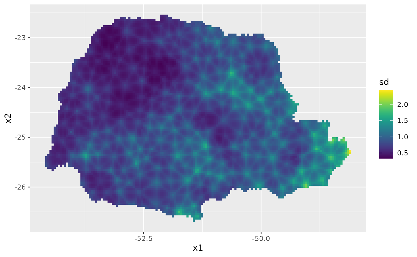

An example with replicates

For this example we will simulate a data with replicates. We will use the same example considered in the Rational approximation with the rSPDE package vignette (the only difference is the way the data is organized). We also refer the reader to this vignette for a description of the function matern.operators(), along with its methods (for instance, the simulate() method).

Simulating the data

Let us consider a simple Gaussian linear model with 30 independent replicates of a latent spatial field $x(\mathbf{s})$, observed at the same $m$ locations, $\{\mathbf{s}_1 , \ldots , \mathbf{s}_m \}$, for each replicate. For each $i = 1,\ldots,m,$ we have

$$\begin{align} y_i &= x_1(\mathbf{s}_i)+\varepsilon_i,\\ \vdots &= \vdots\\ y_{i+29m} &= x_{30}(\mathbf{s}_i) + \varepsilon_{i+29m}, \end{align}$$

where $\varepsilon_1,\ldots,\varepsilon_{30m}$ are iid normally distributed with mean 0 and standard deviation 0.1.

We use the basis function representation of $x(\cdot)$ to define the $A$ matrix linking the point locations to the mesh. We also need to account for the fact that we have 30 replicates at the same locations. To this end, the $A$ matrix we need can be generated by spde.make.A() function. The reason being that we are sampling $x(\cdot)$ directly and not the latent vector described in the introduction of the Rational approximation with the rSPDE package vignette.

We begin by creating the mesh:

m <- 200
loc_2d_mesh <- matrix(runif(m * 2), m, 2)
mesh_2d <- fm_mesh_2d(
  loc = loc_2d_mesh,
  cutoff = 0.05,
  offset = c(0.1, 0.4),
  max.edge = c(0.05, 0.5)
)
plot(mesh_2d, main = "")
points(loc_2d_mesh[, 1], loc_2d_mesh[, 2])

We then compute the $A$ matrix, which is needed for simulation, and connects the observation locations to the mesh. To this end we will use the spde.make.A() helper function, which is a wrapper that uses the functions fm_basis(), fm_block() and fm_row_kron() from the fmesher package.

n.rep <- 30
A <- spde.make.A(
  mesh = mesh_2d,
  loc = loc_2d_mesh,
  index = rep(1:m, times = n.rep),
  repl = rep(1:n.rep, each = m)
)

Notice that for the simulated data, we should use the $A$ matrix from spde.make.A() function instead of the rspde.make.A() function.

We will now simulate a latent process with standard deviation $\sigma=1$ and range $0.1$. We will use $\nu=0.5$ so that the model has an exponential covariance function. To this end we create a model object with the matern.operators() function:

nu <- 0.5
sigma <- 1
range <- 0.1
kappa <- sqrt(8 * nu) / range
tau <- sqrt(gamma(nu) / (sigma^2 * kappa^(2 * nu) * (4 * pi) * gamma(nu + 1)))
d <- 2
operator_information <- matern.operators(
  mesh = mesh_2d,
  nu = nu,
  range = range,
  sigma = sigma,
  m = 2,
  parameterization = "matern"
)

More details on this function can be found at the Rational approximation with the rSPDE package vignette.

To simulate the latent process all we need to do is to use the simulate() method on the operator_information object. We then obtain the simulated data $y$ by connecting with the $A$ matrix and adding the gaussian noise.

set.seed(1)
u <- simulate(operator_information, nsim = n.rep)
y <- as.vector(A %*% as.vector(u)) +
  rnorm(m * n.rep) * 0.1

The first replicate of the simulated random field as well as the observation locations are shown in the following figure.

proj <- fm_evaluator(mesh_2d, dims = c(100, 100))

df_field <- data.frame(x = proj$lattice$loc[,1],
                        y = proj$lattice$loc[,2],
                        field = as.vector(fm_evaluate(proj, 
                        field = as.vector(u[, 1]))),
                        type = "field")

df_loc <- data.frame(x = loc_2d_mesh[, 1],
                      y = loc_2d_mesh[, 2],
                      field = y[1:m],
                      type = "locations")
df_plot <- rbind(df_field, df_loc)

ggplot(df_plot) + aes(x = x, y = y, fill = field) +
        facet_wrap(~type) + xlim(0,1) + ylim(0,1) + 
        geom_raster(data = df_field) +
        geom_point(data = df_loc, aes(colour = field),
        show.legend = FALSE) + 
        scale_fill_viridis() + scale_colour_viridis()

## Warning: Removed 7648 rows containing missing values or values outside the scale range
## (`geom_raster()`).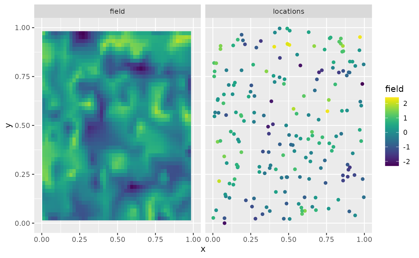

Fitting the R-INLA rSPDE model

Let us then use the rational SPDE approach to fit the data.

We begin by creating the $A$ matrix and index with replicates, and the inla.stack object. It is important to notice that since we have replicates we should provide the index and repl arguments for rspde.make.A() function, and also the argument n.repl in rspde.make.index() function. They behave identically as in their R-INLA’s counterparts, namely, inla.spde.make.A() and inla.make.index().

Abar.rep <- rspde.make.A(
  mesh = mesh_2d, loc = loc_2d_mesh, index = rep(1:m, times = n.rep),
  repl = rep(1:n.rep, each = m)
)
mesh.index.rep <- rspde.make.index(
  name = "field", mesh = mesh_2d,
  n.repl = n.rep
)

st.dat.rep <- inla.stack(
  data = list(y = y),
  A = Abar.rep,
  effects = mesh.index.rep
)

We now create the model object.

rspde_model.rep <- rspde.matern(mesh = mesh_2d, parameterization = "spde") 

Finally, we create the formula and fit. It is extremely important not to forget the replicate argument when building the formula as inla() function will not produce warning and might fit some meaningless model.

f.rep <-
  y ~ -1 + f(field,
    model = rspde_model.rep,
    replicate = field.repl
  )
rspde_fit.rep <-
  inla(f.rep,
    data = inla.stack.data(st.dat.rep),
    family = "gaussian",
    control.predictor =
      list(A = inla.stack.A(st.dat.rep))
  )

We can get the summary:

summary(rspde_fit.rep)

## Time used:
##     Pre = 0.316, Running = 175, Post = 3.29, Total = 178 
## Random effects:
##   Name     Model
##     field CGeneric
## 
## Model hyperparameters:
##                                          mean    sd 0.025quant 0.5quant
## Precision for the Gaussian observations 89.17 4.723      80.01    89.12
## Theta1 for field                        -2.98 0.061      -3.07    -2.99
## Theta2 for field                         3.04 0.038       2.96     3.04
## Theta3 for field                        -1.62 0.028      -1.68    -1.61
##                                         0.975quant  mode
## Precision for the Gaussian observations      98.60 89.20
## Theta1 for field                             -2.84 -3.02
## Theta2 for field                              3.11  3.04
## Theta3 for field                             -1.57 -1.60
## 
## Marginal log-Likelihood:  -4480.38 
##  is computed 
## Posterior summaries for the linear predictor and the fitted values are computed
## (Posterior marginals needs also 'control.compute=list(return.marginals.predictor=TRUE)')

and the summary in the user’s scale:

result_fit_rep <- rspde.result(rspde_fit.rep, "field", rspde_model.rep)
summary(result_fit_rep)

##             mean         sd 0.025quant   0.5quant 0.975quant       mode
## tau    0.0509708 0.00314822  0.0464376  0.0504191  0.0584011  0.0485051
## kappa 20.8913000 0.78425900 19.4017000 20.8730000 22.4812000 20.8314000
## nu     0.6627170 0.01524940  0.6290380  0.6644800  0.6876170  0.6715310

result_df <- data.frame(
  parameter = c("tau", "kappa", "nu"),
  true = c(tau, kappa, nu),
  mean = c(
    result_fit_rep$summary.tau$mean,
    result_fit_rep$summary.kappa$mean,
    result_fit_rep$summary.nu$mean
  ),
  mode = c(
    result_fit_rep$summary.tau$mode,
    result_fit_rep$summary.kappa$mode,
    result_fit_rep$summary.nu$mode
  )
)
print(result_df)

##   parameter        true        mean        mode
## 1       tau  0.08920621  0.05097077  0.04850511
## 2     kappa 20.00000000 20.89126338 20.83143479
## 3        nu  0.50000000  0.66271694  0.67153114

An example with a non-stationary model

It is also possible to consider models in which $\sigma$ (std. deviation) and $\rho$ (range parameter) are non-stationary. One can also use the parameterization in terms of the SPDE parameters $\kappa$ and $\tau$.

An example of such a model is given in the vignette inlabru implementation of the rational SPDE approach.

Further options of the rSPDE-INLA implementation

We will now discuss some of the arguments that were introduced in our R-INLA implementation of the rational approximation that are not present in R-INLA’s standard SPDE implementation.

In each case we will provide an illustrative example.

Changing the upper bound for the smoothness parameter

When we fit a rspde.matern() model we need to provide an upper bound for the smoothness parameter $\nu$. The reason for that is that the sparsity of the precision matrix should be kept fixed during R-INLA’s estimation and the higher the value of $\nu$ the denser the precision matrix gets.

This means that the higher the value of $\nu$, the higher the computational cost to fit the model. Therefore, ideally, want to choose an upper bound for $\nu$ as small as possible.

To change the value of the upper bound for the smoothness parameter, we must change the argument nu.upper.bound. The default value for nu.upper.bound is 4. Other common choices for nu.upper.bound are 2 and 1.

It is clear from the discussion above that the smaller the value of nu.upper.bound the faster the estimation procedure will be.

However, if we choose a value of nu.upper.bound which is too low, the “correct” value of $\nu$ might not belong to the interval $(0,\nu_{UB})$, where $\nu_{UB}$ is the value of nu.upper.bound. Hence, one might be forced to increase nu.upper.bound and estimate again, which, obviously will increase the computational cost as we will need to do more than one estimation.

Let us illustrate by considering the same model we considered above for the precipitation in Paraná region in Brazil and consider nu.upper.bound equal to 2, which is generally a good choice for nu.upper.bound.

We simply use the function rspde.matern() with the argument nu.upper.bound set to 2:

rspde_model_2 <- rspde.matern(mesh = prmesh, nu.upper.bound = 2)

Since we are considering the default rspde.order, the $A$ matrix and the mesh index objects are the same as the previous ones. Let us then update the formula and fit the model:

f.s.2 <- y ~ -1 + Intercept + f(seaDist, model = "rw1") +
  f(field, model = rspde_model_2)

rspde_fit_2 <- inla(f.s.2,
  family = "Gamma", data = inla.stack.data(stk.dat),
  verbose = FALSE,
  control.inla = list(int.strategy = "eb"),
  control.predictor = list(A = inla.stack.A(stk.dat), compute = TRUE)
)

Let us see the summary of the fit:

summary(rspde_fit_2)

## Time used:
##     Pre = 0.301, Running = 9.05, Post = 0.171, Total = 9.52 
## Fixed effects:
##            mean    sd 0.025quant 0.5quant 0.975quant  mode kld
## Intercept 1.943 0.044      1.857    1.943      2.029 1.943   0
## 
## Random effects:
##   Name     Model
##     seaDist RW1 model
##    field CGeneric
## 
## Model hyperparameters:
##                                                   mean      sd 0.025quant
## Precision-parameter for the Gamma observations   13.94    1.01      12.06
## Precision for seaDist                          7716.49 4844.25    2184.74
## Theta1 for field                                 -4.52    4.51     -14.87
## Theta2 for field                                  2.30    1.29       0.29
## Theta3 for field                                  2.79    3.87      -3.13
##                                                0.5quant 0.975quant    mode
## Precision-parameter for the Gamma observations    13.90      16.03   13.82
## Precision for seaDist                           6517.97   20397.52 4704.12
## Theta1 for field                                  -3.96       2.38   -1.09
## Theta2 for field                                   2.15       5.25    1.41
## Theta3 for field                                   2.31      11.67   -0.14
## 
## Marginal log-Likelihood:  -1258.37 
##  is computed 
## Posterior summaries for the linear predictor and the fitted values are computed
## (Posterior marginals needs also 'control.compute=list(return.marginals.predictor=TRUE)')

Let us compare with the cost from the previous fit, with the default value of nu.upper.bound of 4:

# nu.upper.bound = 4
rspde_fit$cpu.used

##        Pre    Running       Post      Total 
##  0.5479393 25.3725297  0.2105370 26.1310060

# nu.upper.bound = 2
rspde_fit_2$cpu.used

##       Pre   Running      Post     Total 
## 0.3013361 9.0490553 0.1714978 9.5218892

We can see that the fit for nu.upper.bound equal to 2 was considerably faster.

Finally, let us get the result results for the field and see the estimate of $\nu$:

result_fit_2 <- rspde.result(rspde_fit_2, "field", rspde_model_2)
summary(result_fit_2)

##           mean        sd  0.025quant  0.5quant 0.975quant        mode
## tau    1.26253  6.735090 9.50608e-11 0.0216991   10.27040 9.50608e-11
## kappa 28.30650 79.988500 1.35537e+00 8.2756400  184.45300 2.56325e+00
## nu     1.44354  0.655293 8.72555e-02 1.8009400    1.99993 1.99999e+00

Changing the order of the rational approximation

To change the order of the rational approximation all we have to do is set the argument rspde.order to the desired value. The current available possibilities are 1,2,3,…, up to 8.

The higher the order of the rational approximation, the more accurate the results will be, however, the higher the computational cost will be.

The default rspde.order of 2 is generally a good choice and reasonably accurate. See the vignette Rational approximation with the rSPDE package for further details on the order of the rational approximation and some comparison with the Matérn covariance.

Let us fit the above model with the covariance-based rational approximation of order 3. Since we are changing the order of the rational approximation, that is, we are changing the rspde.order argument, we need to recompute the $A$ matrix and the mesh index. Therefore, we proceed as follows:

• We build a new model:

rspde_model_order_3 <- rspde.matern(mesh = prmesh, 
  rspde.order = 3,
  nu.upper.bound = 2
)

• We create a new $A$ matrix:

Abar_3 <- rspde.make.A(mesh = prmesh, loc = coords, rspde.order = 3)

• We create a new index:

mesh.index.3 <- rspde.make.index(
  name = "field", mesh = prmesh,
  rspde.order = 3
)

Now the remaining steps are the same as before:

stk.dat.3 <- inla.stack(
  data = list(y = Y), A = list(Abar_3, 1), tag = "est",
  effects = list(
    c(
      mesh.index.3
    ),
    list(
      long = inla.group(coords[, 1]),
      lat = inla.group(coords[, 2]),
      seaDist = inla.group(seaDist),
      Intercept = 1
    )
  )
)

f.s.3 <- y ~ -1 + Intercept + f(seaDist, model = "rw1") +
  f(field, model = rspde_model_order_3)

rspde_fit_order_3 <- inla(f.s.3,
  family = "Gamma", data = inla.stack.data(stk.dat.3),
  verbose = FALSE,
  control.inla = list(int.strategy = "eb"),
  control.predictor = list(A = inla.stack.A(stk.dat.3), compute = TRUE)
)

Let us see the summary:

summary(rspde_fit_order_3)

## Time used:
##     Pre = 0.282, Running = 19.8, Post = 0.109, Total = 20.2 
## Fixed effects:
##            mean    sd 0.025quant 0.5quant 0.975quant  mode kld
## Intercept 1.943 0.043      1.858    1.943      2.028 1.943   0
## 
## Random effects:
##   Name     Model
##     seaDist RW1 model
##    field CGeneric
## 
## Model hyperparameters:
##                                                   mean       sd 0.025quant
## Precision-parameter for the Gamma observations   13.97    1.009     12.044
## Precision for seaDist                          7905.18 4799.068   2388.021
## Theta1 for field                                 -3.55    2.776    -10.007
## Theta2 for field                                  1.85    0.647      0.835
## Theta3 for field                                  1.95    2.380     -1.541
##                                                0.5quant 0.975quant    mode
## Precision-parameter for the Gamma observations    13.95   1.60e+01   13.93
## Precision for seaDist                           6726.52   2.05e+04 4949.89
## Theta1 for field                                  -3.17   5.12e-01   -1.25
## Theta2 for field                                   1.78   3.32e+00    1.41
## Theta3 for field                                   1.63   7.48e+00   -0.01
## 
## Marginal log-Likelihood:  -1259.04 
##  is computed 
## Posterior summaries for the linear predictor and the fitted values are computed
## (Posterior marginals needs also 'control.compute=list(return.marginals.predictor=TRUE)')

We can see in the above summary that the computational cost significantly increased. Let us compare the cost of having rspde.order=3 and nu.upper.bound=2 with the cost of having rspde.order=2 and nu.upper.bound=4:

# nu.upper.bound = 4
rspde_fit$cpu.used

##        Pre    Running       Post      Total 
##  0.5479393 25.3725297  0.2105370 26.1310060

# nu.upper.bound = 2
rspde_fit_order_3$cpu.used

##        Pre    Running       Post      Total 
##  0.2817223 19.7943769  0.1087847 20.1848838

One can check the order of the rational approximation by using the rational.order() function. It also allows another way to change the order of the rational order, by using the corresponding rational.order<-() function.

The rational.order() and rational.order<-() functions can be applied to the inla.rspde object, to the A matrix and to the index objects.

Here to check the models:

rational.order(rspde_model)

## [1] 2

rational.order(rspde_model_order_3)

## [1] 3

Here to check the A matrices:

rational.order(Abar)

## [1] 2

rational.order(Abar_3)

## [1] 3

Here to check the indexes:

rational.order(mesh.index)

## [1] 2

rational.order(mesh.index.3)

## [1] 3

Let us now change the order of the rspde_model object to be 1:

rational.order(rspde_model) <- 1
rational.order(Abar) <- 1
rational.order(mesh.index) <- 1

Let us fit this new model:

 f.s.1 <- y ~ -1 + Intercept + f(seaDist, model = "rw1") +
  f(field, model = rspde_model)

stk.dat.1 <- inla.stack(
  data = list(y = Y), A = list(Abar, 1), tag = "est",
  effects = list(
    c(
      mesh.index
    ),
    list(
      long = inla.group(coords[, 1]),
      lat = inla.group(coords[, 2]),
      seaDist = inla.group(seaDist),
      Intercept = 1
    )
  )
)

rspde_fit_order_1 <- inla(f.s.1,
  family = "Gamma", data = inla.stack.data(stk.dat.1),
  verbose = FALSE,
  control.inla = list(int.strategy = "eb"),
  control.predictor = list(A = inla.stack.A(stk.dat.1), compute = TRUE)
)

Here is the summary:

summary(rspde_fit_order_1)

## Time used:
##     Pre = 0.296, Running = 22.8, Post = 0.0505, Total = 23.2 
## Fixed effects:
##            mean    sd 0.025quant 0.5quant 0.975quant  mode kld
## Intercept 1.924 0.343      1.252    1.924      2.595 1.924   0
## 
## Random effects:
##   Name     Model
##     seaDist RW1 model
##    field CGeneric
## 
## Model hyperparameters:
##                                                     mean       sd 0.025quant
## Precision-parameter for the Gamma observations    14.030 9.76e-01     12.149
## Precision for seaDist                          41353.472 6.63e+04   4685.718
## Theta1 for field                                   0.857 1.90e-01      0.502
## Theta2 for field                                  -1.728 9.54e-01     -3.742
## Theta3 for field                                  -3.055 1.15e+00     -5.240
##                                                 0.5quant 0.975quant     mode
## Precision-parameter for the Gamma observations    14.016   1.60e+01   14.034
## Precision for seaDist                          22655.135   1.99e+05 9971.078
## Theta1 for field                                   0.851   1.25e+00    0.824
## Theta2 for field                                  -1.682  -3.00e-03   -1.461
## Theta3 for field                                  -3.082  -7.12e-01   -3.199
## 
## Marginal log-Likelihood:  -1255.43 
##  is computed 
## Posterior summaries for the linear predictor and the fitted values are computed
## (Posterior marginals needs also 'control.compute=list(return.marginals.predictor=TRUE)')

Estimating models with fixed smoothness

We can fix the smoothness, say $\nu$, of the model by providing a non-NULL positive value for nu.

When the smoothness, $\nu$, is fixed, we can have two possibilities:

• $\alpha = \nu + d/2$ is integer;

• $\alpha = \nu + d/2$ is not integer.

The first case, i.e., when $\alpha$ is integer, has less computational cost. Furthermore, the $A$ matrix is different than the $A$ matrix for the non-integer $\alpha$.

The $A$ matrix is the same for all values of $\nu$ such that $\alpha$ is integer. So, the $A$ matrix for these cases only need to be computed once. The same holds for the index obtained from the rspde.make.index() function.

In the second case the $A$ matrix only depends on the order of the rational approximation and not on $\nu$. Therefore, if the matrix $A$ has already been computed for some rspde.order, then the $A$ matrix will be same for all the values of $\nu$ such that $\alpha$ is non-integer for that rspde.order. The same holds for the index obtained from the rspde.make.index() function.

If $\nu$ is fixed, we have that the parameters returned by R-INLA are $$\kappa = \exp(\theta_1)\quad\hbox{and}\quad\tau = \exp(\theta_2).$$ We will now provide illustrations for both scenarios. It is also noteworthy that just as for the case in which we estimate $\nu$, we can also change the order of the rational approximation by changing the value of rspde.order. For both illustrations with fixed $\nu$ below, we will only consider the order of the rational approximation of 2, that is, the default order.

Estimating models with fixed smoothness and non-integer $\alpha$

Recall that: $$\nu = \nu_{UB}\Big(\frac{\exp(\theta_3)}{1+\exp(\theta_3)}\Big).$$ Thus, to illustrate, let us consider a fixed $\nu$ given by the mean of $\nu$ obtained from the first model we considered in this vignette, namely, the fit given by rspde_fit, which is approximately $\nu = 1.21$.

Notice that for this $\nu$, the value of $\alpha$ is non-integer, so we can use the $A$ matrix and the index of the first fitted model, which is also of order 2.

Therefore, all we have to do is build a new model in which we set nu to 1.21:

rspde_model_fix <- rspde.matern(mesh = prmesh, rspde.order = 2,
  nu = 1.21
)

Let us now fit the model:

f.s.fix <- y ~ -1 + Intercept + f(seaDist, model = "rw1") +
  f(field, model = rspde_model_fix)

rspde_fix <- inla(f.s.fix,
  family = "Gamma", data = inla.stack.data(stk.dat),
  verbose = FALSE,
  control.inla = list(int.strategy = "eb"),
  control.predictor = list(A = inla.stack.A(stk.dat), compute = TRUE)
)

Here we have the summary:

summary(rspde_fix)

## Time used:
##     Pre = 0.27, Running = 6.09, Post = 0.0599, Total = 6.42 
## Fixed effects:
##            mean    sd 0.025quant 0.5quant 0.975quant  mode kld
## Intercept 1.943 0.043      1.859    1.943      2.027 1.943   0
## 
## Random effects:
##   Name     Model
##     seaDist RW1 model
##    field CGeneric
## 
## Model hyperparameters:
##                                                   mean       sd 0.025quant
## Precision-parameter for the Gamma observations   13.90    1.008     12.024
## Precision for seaDist                          7773.39 4725.762   2314.317
## Theta1 for field                                 -1.72    0.370     -2.449
## Theta2 for field                                  1.50    0.288      0.925
##                                                0.5quant 0.975quant    mode
## Precision-parameter for the Gamma observations    13.87     15.990   13.80
## Precision for seaDist                           6617.86  20128.715 4861.17
## Theta1 for field                                  -1.72     -0.993   -1.73
## Theta2 for field                                   1.50      2.060    1.50
## 
## Marginal log-Likelihood:  -1260.29 
##  is computed 
## Posterior summaries for the linear predictor and the fitted values are computed
## (Posterior marginals needs also 'control.compute=list(return.marginals.predictor=TRUE)')

Now, the summary in the original scale:

result_fix <- rspde.result(rspde_fix, "field", rspde_model_fix)
summary(result_fix)

##          mean        sd 0.025quant 0.5quant 0.975quant     mode
## tau   0.19096 0.0724558  0.0869201 0.178348   0.367987 0.155687
## kappa 4.64438 1.3528600  2.5339100 4.461890   7.809680 4.116610

Estimating models with fixed smoothness and integer $\alpha$

Since we are in dimension $d=2$, and $\nu>0$, the smallest value of $\nu$ that makes $\alpha = \nu + 1$ an integer is $\nu=1$. This value is also close to the estimated mean of the first model we fitted and enclosed by the posterior marginal density of $\nu$ for the first fit. Therefore, let us fit the model with $\nu=1$.

To this end we need to compute a new $A$ matrix:

Abar.int <- rspde.make.A(
  mesh = prmesh, loc = coords,
  nu = 1
)

a new index:

mesh.index.int <- rspde.make.index(
  name = "field", mesh = prmesh,
  nu = 1
)

create a new model (remember to set nu=1):

rspde_model_fix_int1 <- rspde.matern(mesh = prmesh,
  nu = 1)

The remaining is standard:

stk.dat.int <- inla.stack(
  data = list(y = Y), A = list(Abar.int, 1), tag = "est",
  effects = list(
    c(
      mesh.index.int
    ),
    list(
      long = inla.group(coords[, 1]),
      lat = inla.group(coords[, 2]),
      seaDist = inla.group(seaDist),
      Intercept = 1
    )
  )
)

f.s.fix.int.1 <- y ~ -1 + Intercept + f(seaDist, model = "rw1") +
  f(field, model = rspde_model_fix_int1)

rspde_fix_int_1 <- inla(f.s.fix.int.1,
  family = "Gamma",
  data = inla.stack.data(stk.dat.int), verbose = FALSE,
  control.inla = list(int.strategy = "eb"),
  control.predictor = list(
    A = inla.stack.A(stk.dat.int),
    compute = TRUE
  )
)

Let us check the summary:

summary(rspde_fix_int_1)

## Time used:
##     Pre = 0.274, Running = 1, Post = 0.0346, Total = 1.31 
## Fixed effects:
##            mean    sd 0.025quant 0.5quant 0.975quant  mode kld
## Intercept 1.943 0.044      1.856    1.943       2.03 1.943   0
## 
## Random effects:
##   Name     Model
##     seaDist RW1 model
##    field CGeneric
## 
## Model hyperparameters:
##                                                   mean       sd 0.025quant
## Precision-parameter for the Gamma observations   13.90    1.006     12.031
## Precision for seaDist                          7958.14 5019.149   2350.275
## Theta1 for field                                 -1.22    0.329     -1.870
## Theta2 for field                                  1.38    0.309      0.773
##                                                0.5quant 0.975quant    mode
## Precision-parameter for the Gamma observations    13.86     15.991   13.79
## Precision for seaDist                           6692.60  21174.366 4844.24
## Theta1 for field                                  -1.22     -0.573   -1.21
## Theta2 for field                                   1.38      1.988    1.38
## 
## Marginal log-Likelihood:  -1260.09 
##  is computed 
## Posterior summaries for the linear predictor and the fitted values are computed
## (Posterior marginals needs also 'control.compute=list(return.marginals.predictor=TRUE)')

and check the summary in the user’s scale:

rspde_result_int <- rspde.result(rspde_fix_int_1, "field", rspde_model_fix_int1)
summary(rspde_result_int)

##           mean       sd 0.025quant 0.5quant 0.975quant     mode
## tau   0.312027 0.104304   0.155051 0.296209   0.560862 0.265598
## kappa 4.164210 1.306180   2.178300 3.970420   7.263620 3.597640

Changing the priors

We begin by recalling that the fitted rSPDE model in R-INLA contains the parameters $\textrm{Theta1}$, $\textrm{Theta2}$ and $\textrm{Theta3}$. Let, again, $\theta_1 = \textrm{Theta1}$, $\theta_2=\textrm{Theta2}$ and $\theta_3=\textrm{Theta3}$. In terms of the SPDE $$(\kappa^2 I - \Delta)^{\alpha/2}(\tau u) = \mathcal{W},$$ where $\alpha = \nu + d/2$.

We also have the range parameter $\rho = \frac{\sqrt{8\nu}}{\kappa}$ and the standard deviation $\sigma = \sqrt{\frac{\Gamma(\nu)}{\tau^2 \kappa^{2\nu}(4\pi)^{d/2}\Gamma(\nu + d/2)}}$.

Changing the priors of $\tau$ and $\kappa$

We begin by dealing with $\tau$ and $\kappa$.

We have that $$\tau = \exp(\theta_1),\quad \kappa = \exp(\theta_2).$$ The rspde.matern() function assumes a lognormal prior distribution for $\tau$ and $\kappa$. This prior distribution is obtained by assuming that $\theta_1$ and $\theta_2$ follow normal distributions. By default we assume $\theta_1$ and $\theta_2$ to be independent and to follow normal distributions $\theta_1\sim N(\log(\tau_0), 10)$ and $\theta_2\sim N(\log(\kappa_0), 10)$.

$\kappa_0$ is suitably defined in terms of the mesh and $\tau_0$ is defined in terms of $\kappa_0$ and on the prior of the smoothness parameter.

If one wants to define the prior $$\theta_1 \sim N(\text{mean_theta_1}, \text{sd_theta_1}),$$ one can simply set the argument prior.tau = list(meanlog=mean_theta_1, sdlog=sd_theta_1). Analogously, to define the prior $$\theta_2 \sim N(\text{mean_theta_2}, \text{sd_theta_2}),$$ one can set the argument prior.kappa = list(meanlog=mean_theta_2, sdlog=sd_theta_2).

It is important to mention that, by default, the initial values of $\tau$ and $\kappa$ are $\exp(\text{mean_theta_1})$ and $\exp(\text{mean_theta_2})$, respectively. So, if the user does not change these parameters, and also does not change the initial values, the initial values of $\tau$ and $\kappa$ will be, respectively, $\tau_0$ and $\kappa_0$.

If one sets prior.tau = list(meanlog=mean_theta_1), the prior for $\theta_1$ will be $$\theta_1 \sim N(\text{mean_theta_1}, 1),$$ whereas, if one sets, prior.tau = list(sdlog=sd_theta_1), the prior will be $$\theta_1 \sim N(\log(\tau_0), \text{sd_theta_1}).$$ Analogously, if one sets prior.kappa = list(meanlog=mean_theta_2), the prior for $\theta_2$ will be $$\theta_2 \sim N(\text{mean_theta_2}, 1),$$ whereas, if one sets, prior.kappa = list(sdlog=sd_theta_2), the prior will be $$\theta_2 \sim N(\log(\kappa_0), \text{sd_theta_2}).$$

Changing the priors of $\rho$ (range) and $\sigma$ (std. dev.)

Let us now consider the priors for the range, $\rho$, and std. deviation, $\sigma$. This parameterization is used with the argument parameterization = "matern", which is the default.

In this case, we have that $$\sigma = \exp(\theta_1),\quad \rho = \exp(\theta_2).$$ We have two options for prior. By default, which is the option prior.theta.param = "theta", the rspde.matern() function assumes a lognormal prior distribution for $\sigma$ and $\rho$. This prior distribution is obtained by assuming that $\theta_1$ and $\theta_2$ follow normal distributions. By default we assume $\theta_1$ and $\theta_2$ to be independent and to follow normal distributions $\theta_1\sim N(\log(\sigma_0), 10)$ and $\theta_2\sim N(\log(\rho_0), 10)$.

$\rho_0$ is suitably defined in terms of the mesh and $\sigma_0$ is defined in terms of $\rho_0$ and on the prior of the smoothness parameter.

Similarly to the priors of $\tau$ and $\kappa$, if one wants to define the prior $$\theta_1 \sim N(\text{mean_theta_1}, \text{sd_theta_1}),$$ one can simply set the argument prior.tau = list(meanlog=mean_theta_1, sdlog=sd_theta_1). Analogously, to define the prior $$\theta_2 \sim N(\text{mean_theta_2}, \text{sd_theta_2}),$$ one can set the argument prior.kappa = list(meanlog=mean_theta_2, sdlog=sd_theta_2).

Another option is to set prior.theta.param = "spde". In this case, a change of variables is performed. So, we assume a lognormal prior on $\tau$ and $\kappa$. Then, by the relations $\rho = \frac{\sqrt{8\nu}}{\kappa}$ and $\sigma = \sqrt{\frac{\Gamma(\nu)}{\tau^2 \kappa^{2\nu}(4\pi)^{d/2}\Gamma(\nu + d/2)}}$, we obtain a prior for $\rho$ and $\sigma$.

Changing the prior of $\nu$

Finally, let us consider the smoothness parameter $\nu$.

By default, we assume that $\nu$ follows a beta distribution on the interval $(0,\nu_{UB})$, where $\nu_{UB}$ is the upper bound for $\nu$, with mean $\nu_0=\min\{1, \nu_{UB}/2\}$ and variance $\frac{\nu_0(\nu_{UB}-\nu_0)}{1+\phi_0}$, and we call $\phi_0$ the precision parameter, whose default value is $$\phi_0 = \max\Big\{\frac{\nu_{UB}}{\nu_0}, \frac{\nu_{UB}}{\nu_{UB}-\nu_0}\Big\} + \phi_{inc}.$$ The parameter $\phi_{inc}$ is an increment to ensure that the prior beta density has boundary values equal to zero (where the boundary values are defined either by continuity or by limits). The default value of $\phi_{inc}$ is 1. The value of $\phi_{inc}$ can be changed by changing the argument nu.prec.inc in the rspde.matern() function. The higher the value of $\phi_{inc}$ (that is, the value of nu.prec.inc) the more informative the prior distribution becomes.

Let us denote a beta distribution with support on $(0,\nu_{UB})$, mean $\mu$ and precision parameter $\phi$ by $\mathcal{B}_{\nu_{UB}}(\mu,\phi)$.

If we want $\nu$ to have a prior $$\nu \sim \mathcal{B}_{\nu_{UB}}(\text{nu_1},\text{prec_1}),$$ one simply needs to set prior.nu = list(mean=nu_1, prec=prec_1). If one sets prior.nu = list(mean=nu_1), then $\nu$ will have prior $$\nu \sim \mathcal{B}_{\nu_{UB}}(\text{nu_1},\phi_1),$$ where $$\phi_1 = \max\Big\{\frac{\nu_{UB}}{\text{nu_1}}, \frac{\nu_{UB}}{\nu_{UB}-\text{nu_1}}\Big\} + \text{nu.prec.inc}.$$

Of one sets prior.nu = list(prec=prec_1), then $\nu$ will have prior $$\nu\sim \mathcal{B}_{\nu_{UB}}(\nu_0, \text{prec_1}).$$ It is also noteworthy that we have that, in terms of R-INLA’s parameters,

$$\nu = \nu_{UB}\Big(\frac{\exp(\theta_3)}{1+\exp(\theta_3)}\Big).$$

It is important to mention that, by default, if a beta prior distribution is chosen for the smoothness parameter $\nu$, then the initial value of $\nu$ is the mean of the prior beta distribution. So, if the user does not change this parameter, and also does not change the initial value, the initial value of $\nu$ will be $\min\{1,\nu_{UB}/2\}$.

We also assume that, in terms of R-INLA’s parameters, $$\nu = \nu_{UB}\Big(\frac{\exp(\theta_3)}{1+\exp(\theta_3)}\Big).$$

We can have another possibility of prior distribution for $\nu$, namely, truncated lognormal distribution. The truncated lognormal distribution is defined in the following sense. We assume that $\log(\nu)$ has prior distribution given by a truncated normal distribution with support $(-\infty,\log(\nu_{UB}))$, where $\nu_{UB}$ is the upper bound for $\nu$, with location parameter $\mu_0 =\log(\nu_0)= \log\Big(\min\{1,\nu_{UB}/2\}\Big)$ and scale parameter $\sigma_0 = 1$. More precisely, let $\Phi(\cdot; \mu,\sigma)$ stand for the cumulative distribution function (CDF) of a normal distribution with mean $\mu$ and standard deviation $\sigma$. Then, $\log(\nu)$ has cumulative distribution function given by $$F_{\log(\nu)}(x) = \frac{\Phi(x;\mu_0,\sigma_0)}{\Phi(\nu_{UB})},\quad x\leq \nu_{UB},$$ and $F_{\log(\nu)}(x) = 1$ if $x>\nu_{UB}$. We will call $\mu_0$ and $\sigma_0$ the log-location and log-scale parameters of $\nu$, respectively, and we say that $\log(\nu)$ follows a truncated normal distribution with location parameter $\mu_0$ and scale parameter $\sigma_0$.

To change the prior distribution of $\nu$ to the truncated lognormal distribution, we need to set the argument prior.nu.dist="lognormal".

To change these parameters in the prior distribution to, say, log_nu_1 and log_sigma_1, one can simply set prior.nu = list(loglocation=log_nu_1, logscale=sigma_1).

If one sets prior.nu = list(loglocation=log_nu_1), the prior for $\theta_3$ will be a truncated normal normal distribution with location parameter log_nu_1 and scale parameter 1. Analogously, if one sets, prior.nu = list(logscale=sigma_1), the prior for $\theta_3$ will be a truncated normal distribution with location parameter $\log(\nu_0)= \log\Big(\min\{1,\nu_{UB}/2\}\Big)$ and scale parameter sigma_1.

It is important to mention that, by default, if a truncated lognormal prior distribution is chosen for the smoothness parameter $\nu$, then the initial value of $\nu$ is the exponential of the log-location parameter of $\nu$. So, if the user does not change this parameter, and also does not change the initial value, the initial value of $\nu$ will be $\min\{1,\nu_{UB}/2\}$.

Let us consider an example with the same dataset used in the first model of this vignette where we change the prior distribution of $\nu$ from beta to lognormal.

rspde_model_beta <- rspde.matern(mesh = prmesh, prior.nu.dist = "lognormal")

Since we did not change rspde.order and are not fixing $\nu$, we can use the same $A$ matrix and same index from the first example.

Therefore, all we have to do is update the formula and fit the model:

f.s.beta <- y ~ -1 + Intercept + f(seaDist, model = "rw1") +
  f(field, model = rspde_model_beta)

rspde_fit_beta <- inla(f.s.beta,
  family = "Gamma", data = inla.stack.data(stk.dat),
  verbose = FALSE,
  control.inla = list(int.strategy = "eb"),
  control.predictor = list(A = inla.stack.A(stk.dat), compute = TRUE)
)

We have the summary:

summary(rspde_fit_beta)

## Time used:
##     Pre = 0.286, Running = 34.6, Post = 0.0666, Total = 35 
## Fixed effects:
##            mean    sd 0.025quant 0.5quant 0.975quant  mode kld
## Intercept 1.943 0.043       1.86    1.943      2.027 1.943   0
## 
## Random effects:
##   Name     Model
##     seaDist RW1 model
##    field CGeneric
## 
## Model hyperparameters:
##                                                    mean       sd 0.025quant
## Precision-parameter for the Gamma observations   13.889    1.011     12.008
## Precision for seaDist                          7832.575 4968.017   2357.354
## Theta1 for field                                 -1.987    1.444     -4.871
## Theta2 for field                                  1.541    0.352      0.854
## Theta3 for field                                 -0.705    0.689     -2.044
##                                                0.5quant 0.975quant     mode
## Precision-parameter for the Gamma observations   13.851   1.60e+01   13.773
## Precision for seaDist                          6566.771   2.09e+04 4747.470
## Theta1 for field                                 -1.973   8.13e-01   -1.914
## Theta2 for field                                  1.539   2.24e+00    1.529
## Theta3 for field                                 -0.712   6.70e-01   -0.738
## 
## Marginal log-Likelihood:  -1260.95 
##  is computed 
## Posterior summaries for the linear predictor and the fitted values are computed
## (Posterior marginals needs also 'control.compute=list(return.marginals.predictor=TRUE)')

Also, we can have the summary in the user’s scale:

result_fit_beta <- rspde.result(rspde_fit_beta, "field", rspde_model_beta)
summary(result_fit_beta)

##           mean       sd 0.025quant 0.5quant 0.975quant      mode
## tau   0.368743 0.764071 0.00787605 0.139467    2.20803 0.0158874
## kappa 4.964210 1.796170 2.36305000 4.655940    9.33875 4.1018900
## nu    1.381340 0.572397 0.46304600 1.315680    2.63464 1.1226000

and the plot of the posterior marginal densities

posterior_df_fit_beta <- gg_df(result_fit_beta)

ggplot(posterior_df_fit_beta) + geom_line(aes(x = x, y = y)) + 
facet_wrap(~parameter, scales = "free") + labs(y = "Density")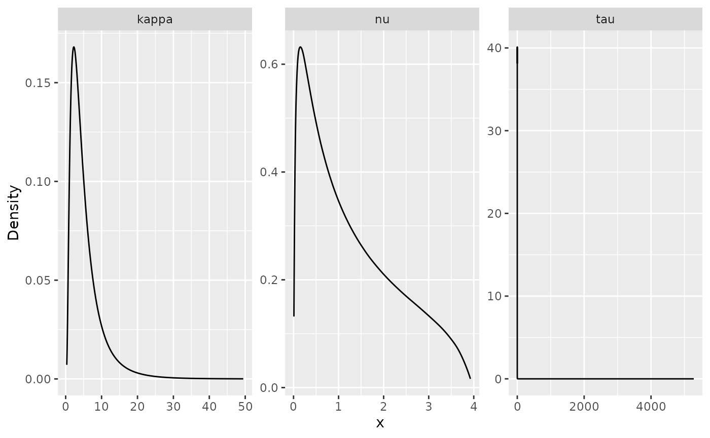

Changing the starting values

The starting values to be used by R-INLA’s optimization algorithm can be changed by setting the arguments start.ltau, start.lkappa and start.nu.

• start.ltau will be the initial value for $\log(\tau)$, that is, the logarithm of $\tau$.

• start.lkappa will be the inital value for $\log(\kappa)$, that is, the logarithm of $\kappa$.

• start.nu will be the initial value for $\nu$. Notice that here the initial value is not on the log scale.

One can change the initial value of one or more parameters.

For instance, let us consider the example with precipitation data, rspde.order=3, but change the initial values to the ones close to the fitted value when considering the default rspde.order (which is 2):

rspde_model_order_3_start <- rspde.matern(mesh = prmesh, rspde.order = 3,
  nu.upper.bound = 2,
  start.lkappa = result_fit$summary.log.kappa$mean,
  start.ltau = result_fit$summary.log.tau$mean,
  start.nu = min(result_fit$summary.nu$mean, 2 - 1e-5)
)

Since we already computed the $A$ matrix and the index for rspde.order=3, all we have to do is to update the formula and fit:

f.s.3.start <- y ~ -1 + Intercept + f(seaDist, model = "rw1") +
  f(field, model = rspde_model_order_3_start)

rspde_fit_order_3_start <- inla(f.s.3.start,
  family = "Gamma",
  data = inla.stack.data(stk.dat.3),
  verbose = FALSE,
  control.inla = list(int.strategy = "eb"),
  control.predictor = list(
    A = inla.stack.A(stk.dat.3),
    compute = TRUE
  )
)

We have the summary:

summary(rspde_fit_order_3_start)

## Time used:
##     Pre = 0.326, Running = 13.8, Post = 0.0757, Total = 14.2 
## Fixed effects:
##            mean    sd 0.025quant 0.5quant 0.975quant  mode kld
## Intercept 1.944 0.051      1.844    1.944      2.044 1.944   0
## 
## Random effects:
##   Name     Model
##     seaDist RW1 model
##    field CGeneric
## 
## Model hyperparameters:
##                                                    mean       sd 0.025quant
## Precision-parameter for the Gamma observations   13.931    0.999     12.080
## Precision for seaDist                          9406.307 6665.775   2610.046
## Theta1 for field                                  0.154    0.361     -0.507
## Theta2 for field                                  0.809    0.431     -0.080
## Theta3 for field                                 -1.353    0.496     -2.371
##                                                0.5quant 0.975quant     mode
## Precision-parameter for the Gamma observations   13.891     16.012   13.803
## Precision for seaDist                          7614.003  27156.208 5229.350
## Theta1 for field                                  0.139      0.909    0.067
## Theta2 for field                                  0.822      1.615    0.884
## Theta3 for field                                 -1.339     -0.417   -1.278
## 
## Marginal log-Likelihood:  -1259.70 
##  is computed 
## Posterior summaries for the linear predictor and the fitted values are computed
## (Posterior marginals needs also 'control.compute=list(return.marginals.predictor=TRUE)')

Changing the type of the rational approximation

We have three rational approximations available. The BRASIL algorithm Hofreither (2021), and two “versions” of the Clenshaw-Lord Chebyshev-Pade algorithm, one with lower bound zero and another with the lower bound given in Bolin, Simas, and Xiong (2023).

The type of rational approximation can be chosen by setting the type.rational.approx argument in the rspde.matern function. The BRASIL algorithm corresponds to the choice brasil, the Clenshaw-Lord Chebyshev pade with zero lower bound and non-zero lower bounds are given, respectively, by the choices chebfun and chebfunLB.

Let us fit a model assigning a brasil rational approximation. We will consider a model with the order of the rational approximation being 1:

rspde_model_brasil <- rspde.matern(prmesh, 
              type.rational.approx = "brasil")

f.s.brasil <- y ~ -1 + Intercept + f(seaDist, model = "rw1") +
  f(field, model = rspde_model_brasil)

rspde_fit_order_1_brasil <- inla(f.s.brasil,
  family = "Gamma", data = inla.stack.data(stk.dat),
  verbose = FALSE,
  control.inla = list(int.strategy = "eb"),
  control.predictor = list(A = inla.stack.A(stk.dat), compute = TRUE)
)

Let us get the summary:

summary(rspde_fit_order_1_brasil)

## Time used:
##     Pre = 0.283, Running = 44, Post = 0.0641, Total = 44.3 
## Fixed effects:
##            mean    sd 0.025quant 0.5quant 0.975quant  mode kld
## Intercept 1.924 0.356      1.227    1.924      2.622 1.924   0
## 
## Random effects:
##   Name     Model
##     seaDist RW1 model
##    field CGeneric
## 
## Model hyperparameters:
##                                                    mean       sd 0.025quant
## Precision-parameter for the Gamma observations    13.84 9.69e-01     11.966
## Precision for seaDist                          36477.45 4.38e+04   6869.804
## Theta1 for field                                   1.12 2.68e-01      0.684
## Theta2 for field                                  -3.18 1.67e+00     -7.061
## Theta3 for field                                  -4.73 1.53e+00     -8.134
##                                                0.5quant 0.975quant     mode
## Precision-parameter for the Gamma observations    13.82   1.58e+01    13.85
## Precision for seaDist                          23749.69   1.49e+05 12601.32
## Theta1 for field                                   1.10   1.72e+00     0.98
## Theta2 for field                                  -2.96  -7.18e-01    -1.82
## Theta3 for field                                  -4.59  -2.19e+00    -3.93
## 
## Marginal log-Likelihood:  -1257.01 
##  is computed 
## Posterior summaries for the linear predictor and the fitted values are computed
## (Posterior marginals needs also 'control.compute=list(return.marginals.predictor=TRUE)')

Finally, similarly to the order of the rational approximation, one can check the order with the rational.type() function, and assign a new type with the rational.type<-() function.

rational.type(rspde_model)

## [1] "chebfun"

rational.type(rspde_model_brasil)

## [1] "brasil"

Let us change the type of the rational approximation on the model with rational approximation of order 3:

rational.type(rspde_model_order_3) <- "brasil"

f.s.3 <- y ~ -1 + Intercept + f(seaDist, model = "rw1") +
  f(field, model = rspde_model_order_3)

rspde_fit_order_3_brasil <- inla(f.s.3,
  family = "Gamma", data = inla.stack.data(stk.dat.3),
  verbose = FALSE,
  control.inla = list(int.strategy = "eb"),
  control.predictor = list(A = inla.stack.A(stk.dat.3), compute = TRUE)
)

Let us get the summary:

summary(rspde_fit_order_3_brasil)

## Time used:
##     Pre = 0.289, Running = 16.1, Post = 0.122, Total = 16.5 
## Fixed effects:
##            mean    sd 0.025quant 0.5quant 0.975quant  mode kld
## Intercept 1.943 0.044      1.857    1.943      2.029 1.943   0
## 
## Random effects:
##   Name     Model
##     seaDist RW1 model
##    field CGeneric
## 
## Model hyperparameters:
##                                                   mean      sd 0.025quant
## Precision-parameter for the Gamma observations   13.94    1.01     12.042
## Precision for seaDist                          7699.86 4620.76   2282.223
## Theta1 for field                                 -3.85    4.05    -13.010
## Theta2 for field                                  2.06    1.09      0.298
## Theta3 for field                                  2.21    3.46     -3.273
##                                                0.5quant 0.975quant     mode
## Precision-parameter for the Gamma observations    13.90      16.01   13.852
## Precision for seaDist                           6587.27   19730.06 4860.861
## Theta1 for field                                  -3.40       2.58   -1.275
## Theta2 for field                                   1.95       4.52    1.408
## Theta3 for field                                   1.84      10.04    0.025
## 
## Marginal log-Likelihood:  -1258.51 
##  is computed 
## Posterior summaries for the linear predictor and the fitted values are computed
## (Posterior marginals needs also 'control.compute=list(return.marginals.predictor=TRUE)')

References

Bolin, David, Alexandre B. Simas, and Zhen Xiong. 2023. “Covariance-Based Rational Approximations of Fractional SPDEs for Computationally Efficient Bayesian Inference.” Journal of Computational and Graphical Statistics.

Hofreither, Clemens. 2021. “An Algorithm for Best Rational Approximation Based on Barycentric Rational Interpolation.” Numerical Algorithms 88 (1): 365–88.

Lindgren, Finn, Håvard Rue, and Johan Lindström. 2011. “An Explicit Link Between Gaussian Fields and Gaussian Markov Random Fields: The Stochastic Partial Differential Equation Approach.” Journal of the Royal Statistical Society. Series B. Statistical Methodology 73 (4): 423–98.