Rational approximation of the Matern fields on intervals and metric graphs

The function is used for computing an approximation, which can be used for inference and simulation, of the fractional SPDE $$(\kappa^2 - \Delta)^{\alpha/2} (\tau u(s)) = W$$ on intervals or metric graphs. Here $W$ is Gaussian white noise, $\kappa$ controls the range, $\alpha = \nu + 1/2$ with $\nu>0$ controls the smoothness and $\tau$ is related to the marginal variances through $$\sigma^2 = \frac{\Gamma(\nu)}{\tau^2\Gamma(\alpha)2\sqrt{\pi}\kappa^{2\nu}}.$$

Usage

matern.rational(
  graph = NULL,
  loc = NULL,
  bc = c("free", "Neumann", "Dirichlet"),
  kappa = NULL,
  range = NULL,
  nu = NULL,
  sigma = NULL,
  tau = NULL,
  alpha = NULL,
  m = 2,
  parameterization = c("matern", "spde"),
  type_rational_approximation = "brasil",
  type_interp = "spline"
)

Arguments

graph: Metric graph object. The default is NULL, which means that a stationary Matern model on the line is created.
loc: Locations where to evaluate the model.
bc: Specifies the boundary conditions. The default is "free" which gives stationary Matern models on intervals. Other options are "Neumann" or "Dirichlet".
kappa: Range parameter
range: practical correlation range
nu: Smoothness parameter
sigma: Standard deviation
tau: Precision parameter
alpha: Smoothness parameter
m: The order of the approximation
parameterization: Which parameterization to use? matern uses range, std. deviation and nu (smoothness). spde uses kappa, tau and alpha. The default is matern.
type_rational_approximation: Method used to compute the coefficients of the rational approximation.
type_interp: Interpolation method for the rational coefficients.

Value

A model object for the the approximation

Examples

s <- seq(from = 0, to = 1, length.out = 101)
kappa <- 20
sigma <- 2
nu <- 0.8
r <- sqrt(8*nu)/kappa #range parameter
op_cov <- matern.rational(loc = s, nu = nu, range = r, sigma = sigma, m = 2, 
parameterization = "matern")
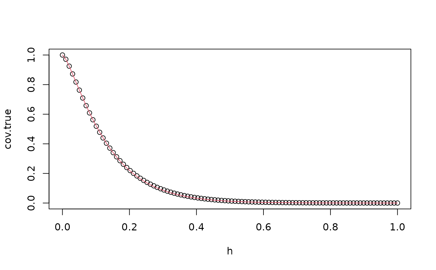
cov.true <- matern.covariance(abs(s-s[1]), kappa = kappa, sigma = sigma, nu = nu)
cov.approx <- op_cov$covariance(ind = 1)

plot(s, cov.true)
lines(s, cov.approx, col = 2)