Precision matrix of stationary Gaussian Matern random fields with integer covariance exponent

rspde.matern.precision.integer.opt is used for computing the precision matrix of stationary Gaussian random fields on \(R^d\) with a Matern covariance function $$C(h) = \frac{\sigma^2}{2^(\nu-1)\Gamma(\nu)} (\kappa h)^\nu K_\nu(\kappa h)$$, where \(\alpha = \nu + d/2\) is a natural number.

Usage

rspde.matern.precision.integer(
  kappa,
  nu,
  tau = NULL,
  sigma = NULL,
  dim,
  fem_mesh_matrices
)

Arguments

kappa

Range parameter of the covariance function.

nu

Shape parameter of the covariance function.

tau

Scale parameter of the covariance function.

sigma

Standard deviation of the covariance function. If tau is not provided, sigma should be provided.

dim

The dimension of the domain

fem_mesh_matrices

A list containing the FEM-related matrices. The list should contain elements c0, g1, g2, g3, etc.

Value

The precision matrix

Examples

set.seed(123)
nobs <- 101
x <- seq(from = 0, to = 1, length.out = nobs)
fem <- rSPDE.fem1d(x)
kappa <- 40
sigma <- 1
d <- 1
nu <- 0.5
tau <- sqrt(gamma(nu) / (kappa^(2 * nu) *
  (4 * pi)^(d / 2) * gamma(nu + d / 2)))
range <- sqrt(8 * nu) / kappa
op_cov <- matern.operators(
  loc_mesh = x, nu = nu, range = range, sigma = sigma,
  d = 1, m = 2, parameterization = "matern"
)
v <- t(rSPDE.A1d(x, 0.5))
c.true <- matern.covariance(abs(x - 0.5), kappa, nu, sigma)
Q <- rspde.matern.precision.integer(
  kappa = kappa, nu = nu, tau = tau, d = 1,
  fem_mesh_matrices = op_cov$fem_mesh_matrices
)
A <- Diagonal(nobs)
c.approx_cov <- A %*% solve(Q, v)

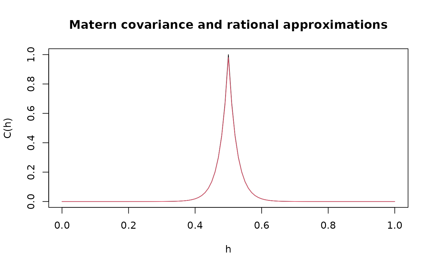
# plot the result and compare with the true Matern covariance
plot(x, matern.covariance(abs(x - 0.5), kappa, nu, sigma),
  type = "l", ylab = "C(h)",
  xlab = "h", main = "Matern covariance and rational approximations"
)
lines(x, c.approx_cov, col = 2)