This is a demonstration of using ngme2 package to fit a
space-time bivariate model. Before use this model, please make sure you
are familiar with the space-time (tensor product) model and bivariate
model separately (Please see Ngme2
space-time model and Ngme2 bivariate
model for more details).
This model is a combination of the previous two, we use the bivariate model as the second part of the tensor product model.
Simulation
## This is ngme2 of version 0.7.1
## - See our homepage: https://davidbolin.github.io/ngme2 for more details.
##
## Attaching package: 'ngme2'## The following object is masked from 'package:stats':
##
## arFirst we specify the two indices for the space-time model. We have 20 time points and 40 mesh locations for space.
time_len = 20
half_bv_len = 50

# specify indices for 2 parts
time_idx = rep(1:time_len, each=half_bv_len*2)
bv_idx = rep(c(1:half_bv_len,1:half_bv_len), time_len)

# group to indicate two different fields for bivariate model
group = rep(rep(c("f1", "f2"), each=half_bv_len),time_len)
Next, we specify the bivariate model using a list, here we consider a bivariate model with two AR(1) processes.
bv_list <- list(
  model="bv",
  sub_models = list(
    f1 = list(
      model="ar1",
      rho=0.5
    ),
    f2 = list(
      model="ar1",
      rho=-0.3
    )
  )
)


mesh_s <- fmesher::fm_mesh_1d(seq(0, 1, length.out=40))

bv_matern_normal_list <- list(
  model="bv_matern_normal",
  mesh = mesh_s,
  group = group,
  sub_models = list(
    f1 = list(
      model="matern"
    ),
    f2 = list(
      model="matern"
    )
  )
)

f_matern_normal <- f(
  map=list(
    time_idx,
    bv_idx
  ),
  model="tp",
  first = list(
    model="ar1", rho=0.6
  ),
  second = bv_matern_normal_list,
  group = group,
  noise=noise_nig(
    mu=-2,
    sigma=1,
    nu=2
  )
)
f_matern_normal
## Model type: Tensor product
## first: AR(1)
## rho = 0.6
## second: Bivariate Matern model (normal noise)
## theta = 0(fixed)
## rho = 0
## sd1 = 1
## sd2 = 1
## f1: Matern
## kappa = 1
## f2: Matern
## kappa = 1
## Noise type: NIG
## Noise parameters:
## mu = -2
## sigma = 1
## nu = 2
bv_matern_nig_list <- list(
  model="bv_matern_nig",
  mesh = mesh_s,
  group = group,
  sub_models = list(
    f1 = list(
      model="matern"
    ),
    f2 = list(
      model="matern"
    )
  ),
  noise = list(
    f1 = noise_nig(),
    f2 = noise_nig()
  )
)

f_matern_nig <- f(
  map=list(
    time_idx,
    bv_idx
  ),
  model="tp",
  first = list(
    model="ar1", rho=0.6
  ),
  second = bv_matern_nig_list,
  group = group,
  noise=noise_nig(
    mu=-2,
    sigma=1,
    nu=2
  )
)
f_matern_nig
## Model type: Tensor product
## first: AR(1)
## rho = 0.6
## second: Bivariate Matern model (NIG noise)
## theta = 0
## rho = 0
## sd1 = 1
## sd2 = 1
## f1: Matern
## kappa = 1
## f2: Matern
## kappa = 1
## Noise type: NIG
## Noise parameters:
## mu = -2
## sigma = 1
## nu = 2Then we specify the full model using the f function,
which is a tensor product model with the first part being an AR(1)
process and the second part being the bivariate model.
f_model <- f(
  map=list(
    time_idx,
    bv_idx
  ),
  model="tp",
  first = list(
    model="ar1", rho=0.6
  ),
  second = bv_list,
  group = group,
  noise=noise_nig(
    mu=-2,
    sigma=1,
    nu=2
  )
)
f_model
## Model type: Tensor product
## first: AR(1)
## rho = 0.6
## second: Bivariate model (non-Gaussian noise)
## theta = 0
## rho = 0
## f1: AR(1)
## rho = 0.5
## f2: AR(1)
## rho = -0.3
## Noise type: NIG
## Noise parameters:
## mu = -2
## sigma = 1
## nu = 2Estimation
Now we turn to estimate the model using simulated data.
bv_list_2 <- list(
  model="bv",
  sub_models = list(
    f1 = list(
      model="ar1"
    ),
    f2 = list(
      model="ar1"
    )
  )
)
nn = length(Y)

fit0 = ngme(
  Y ~ 0 + f(1:nn, model="rw1") +
    f(map=list(
      time_idx, bv_idx
    ),
    model="tp",
    first = list(model="ar1"),
    second = bv_list_2,
    noise=noise_nig()
  ),
  control_opt = control_opt(
    iterations = 10
  ),
  data=data.frame(Y=Y),
  group = group
)
## Starting estimation...
##
## Starting posterior sampling...
## Posterior sampling done!
## Average standard deviation of the posterior W: 1.487386
## Note:
## 1. Use ngme_post_samples(..) to access the posterior samples.
## 2. Use ngme_result(..) to access different latent models.
fit0## *** Ngme object ***
##
## Fixed effects:
## None
##
## Models:
## $field1
## Model type: Random walk (order 1)
## No parameter.
## Noise type: NORMAL
## Noise parameters:
## sigma = 0.716
##
## $field2
## Model type: Tensor product
## first: AR(1)
## rho = 0.219
## second: Bivariate model (non-Gaussian noise)
## theta = -0.278
## rho = -0.159
## f1: AR(1)
## rho = NA
## f2: AR(1)
## rho = NA
## Noise type: NIG
## Noise parameters:
## mu = -0.218
## sigma = 1.21
## nu = 0.76
##
## Measurement noise:
## Noise type: NORMAL
## Noise parameters:
## sigma = 1.23
traceplot(fit0, "field1")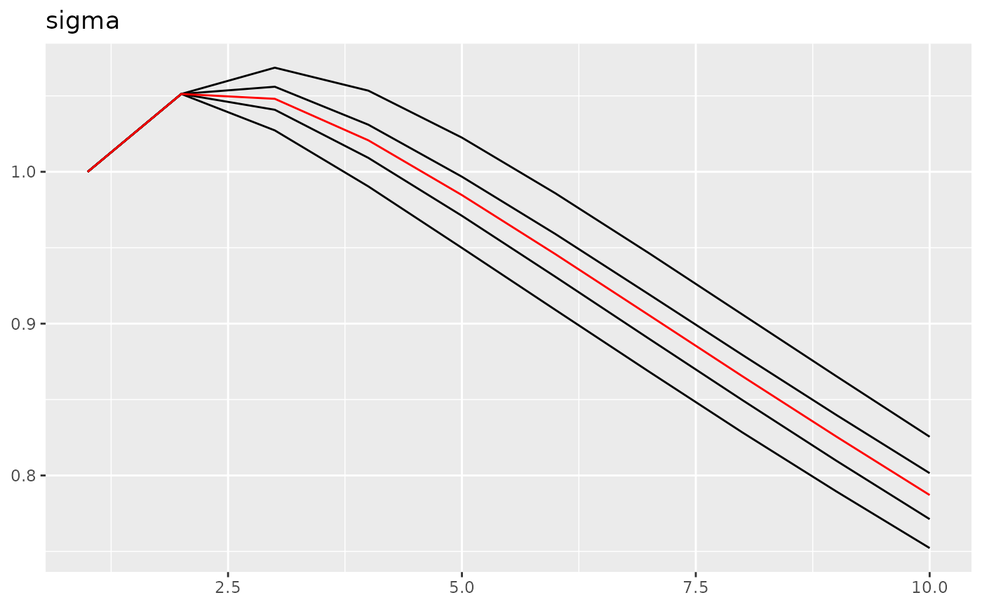
## Last estimates:
## $sigma
## [1] 0.8556059
Here we can see, we get the simulated parameter correctly.