Rational approximations of fractional operators

fractional.operators is used for computing an approximation, which can be used for inference and simulation, of the fractional SPDE $$L^\beta (\tau u(s)) = W.$$ Here $L$ is a differential operator, $\beta>0$ is the fractional power, $\tau$ is a positive scalar or vector that scales the variance of the solution $u$, and $W$ is white noise.

Usage

fractional.operators(L, beta, C, scale.factor, m = 1, tau = 1)

Arguments

L: A finite element discretization of the operator $L$.
beta: The positive fractional power.
C: The mass matrix of the finite element discretization.
scale.factor: A constant $c$ is a lower bound for the the smallest eigenvalue of the non-discretized operator $L$.
m: The order of the rational approximation, which needs to be a positive integer. The default value is 1. Higer values gives a more accurate approximation, which are more computationally expensive to use for inference. Currently, the largest value of m that is implemented is 4.
tau: The constant or vector that scales the variance of the solution. The default value is 1.

Value

fractional.operators returns an object of class "rSPDEobj". This object contains the following quantities:

Pl: The operator $P_l$.
Pr: The operator $P_r$.
C: The mass lumped mass matrix.
Ci: The inverse of C.
m: The order of the rational approximation.
beta: The fractional power.
type: String indicating the type of approximation.
Q: The matrix t(Pl) %*% solve(C,Pl).
type: String indicating the type of approximation.
Pl.factors: List with elements that can be used to assemble $P_l$.
Pr.factors: List with elements that can be used to assemble $P_r$.

Details

The approximation is based on a rational approximation of the fractional operator, resulting in an approximate model on the form $$P_l u(s) = P_r W,$$ where $P_j = p_j(L)$ are non-fractional operators defined in terms of polynomials $p_j$ for $j=l,r$. The order of $p_r$ is given by m and the order of $p_l$ is $m + m_\beta$ where $m_\beta$ is the integer part of $\beta$ if $\beta>1$ and $m_\beta = 1$ otherwise.

The discrete approximation can be written as $u = P_r x$ where $x \sim N(0,Q^{-1})$ and $Q = P_l^T C^{-1} P_l$. Note that the matrices $P_r$ and $Q$ may be be ill-conditioned for $m>1$. In this case, the methods in operator.operations() should be used for operations involving the matrices, since these methods are more numerically stable.

Examples

# Compute rational approximation of a Gaussian process with a
# Matern covariance function on R
kappa <- 10
sigma <- 1
nu <- 0.8

# create mass and stiffness matrices for a FEM discretization
x <- seq(from = 0, to = 1, length.out = 101)
fem <- rSPDE.fem1d(x)

# compute rational approximation of covariance function at 0.5
tau <- sqrt(gamma(nu) / (sigma^2 * kappa^(2 * nu) *
  (4 * pi)^(1 / 2) * gamma(nu + 1 / 2)))
op <- fractional.operators(
  L = fem$G + kappa^2 * fem$C, beta = (nu + 1 / 2) / 2,
  C = fem$C, scale.factor = kappa^2, tau = tau
)

v <- t(rSPDE.A1d(x, 0.5))
c.approx <- Sigma.mult(op, v)

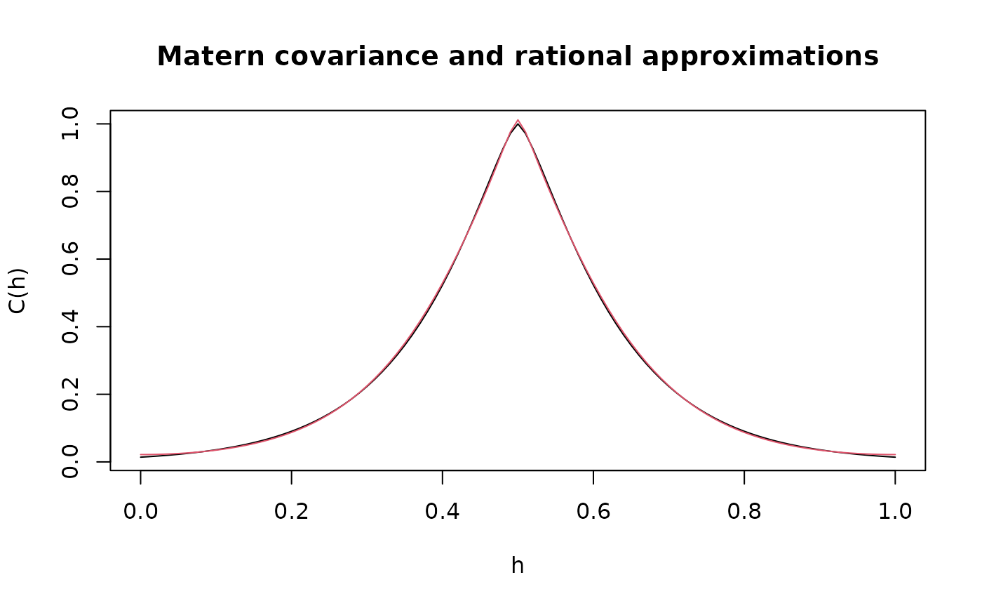
# plot the result and compare with the true Matern covariance
plot(x, matern.covariance(abs(x - 0.5), kappa, nu, sigma),
  type = "l", ylab = "C(h)",
  xlab = "h", main = "Matern covariance and rational approximations"
)
lines(x, c.approx, col = 2)

Usage

Arguments

Value

Details

See also

Examples