Covariance-based approximations of intrinsic fields — intrinsic.matern.operators • rSPDE

intrinsic.matern.operators is used for computing a covariance-based rational SPDE approximation of intrinsic fields on $R^d$ defined through the SPDE $$(-\Delta)^{\beta/2}(\kappa^2-\Delta)^{\alpha/2} (\tau u) = \mathcal{W}$$

Usage

intrinsic.matern.operators(
  kappa,
  tau,
  alpha,
  beta = 1,
  G = NULL,
  C = NULL,
  d = NULL,
  mesh = NULL,
  graph = NULL,
  loc_mesh = NULL,
  m_alpha = 2,
  m_beta = 2,
  compute_higher_order = FALSE,
  return_block_list = FALSE,
  type_rational_approximation = c("brasil", "chebfun", "chebfunLB"),
  fem_mesh_matrices = NULL,
  scaling = NULL,
  opts = NULL
)

Arguments

kappa: range parameter
tau: precision parameter
alpha: Smoothness parameter
beta: Smoothness parameter
G: The stiffness matrix of a finite element discretization of the domain of interest.
C: The mass matrix of a finite element discretization of the domain of interest.
d: The dimension of the domain.
mesh: An inla mesh.
graph: An optional metric_graph object. Replaces d, C and G.
loc_mesh: locations for the mesh for d=1.
m_alpha: The order of the rational approximation for the Matérn part, which needs to be a positive integer. The default value is 2.
m_beta: The order of the rational approximation for the intrinsic part, which needs to be a positive integer. The default value is 2.
compute_higher_order: Logical. Should the higher order finite element matrices be computed?
return_block_list: Logical. For type = "covariance", should the block parts of the precision matrix be returned separately as a list?
type_rational_approximation: Which type of rational approximation should be used? The current types are "brasil", "chebfun" or "chebfunLB".
fem_mesh_matrices: A list containing FEM-related matrices. The list should contain elements c0, g1, g2, g3, etc.
scaling: scaling factor, see details.
opts: options for numerical calulcation of the scaling, see details.

Value

intrinsic.matern.operators returns an object of class "intrinsicCBrSPDEobj". This object is a list including the following quantities:

C: The mass lumped mass matrix.
Ci: The inverse of C.
GCi: The stiffness matrix G times Ci
Q: The precision matrix.
Q_list: A list containing the blocks required to assemble the precision matrix.
alpha: The fractional power of the Matérn part of the operator.
beta: The fractional power of the intrinsic part of the operator.
kappa: Range parameter of the covariance function
tau: Scale parameter of the covariance function.
m_alpha: The order of the rational approximation for the Matérn part.
m_beta: The order of the rational approximation for the intrinsic part.
m: The total number of blocks in the precision matrix.
n: The number of mesh nodes.
d: The dimension of the domain.
type_rational_approximation: String indicating the type of rational approximation.
higher_order: Boolean indicating if higher order FEM-related matrices are computed.
return_block_list: Boolean indicating if the precision matrix is returned as a list with the blocks.
fem_mesh_matrices: A list containing the mass lumped mass matrix, the stiffness matrix and the higher-order FEM-related matrices.
make_A: A function to compute the projection matrix which links the field to observation locations.
variogram: A function to compute the variogram of the model at a specified node.
A: Matrix that sums the components in the approximation to the mesh nodes.
scaling: The scaling used in the intrinsic part of the model.

Details

The covariance operator $$\tau^{-2}(-\Delta)^{\beta}(\kappa^2-\Delta)^{\alpha}$$ is approximated based on rational approximations of the two fractional components. The Laplacians are equipped with homogeneous Neumann boundary conditions. Unless supplied, the scaling is computed as the lowest positive eigenvalue of sqrt(solve(c0))%*%g1%*%sqrt(solve(c0)). opts provides a list of options for the numerical calculation of the scaling factor, which is done using Rspectra::eigs_sym. See the help of that function for details.

Examples

if (requireNamespace("RSpectra", quietly = TRUE)) {
  x <- seq(from = 0, to = 10, length.out = 201)
  beta <- 1
  alpha <- 1
  kappa <- 1
  op <- intrinsic.matern.operators(
    kappa = kappa, tau = 1, alpha = alpha,
    beta = beta, loc_mesh = x, d = 1
  )
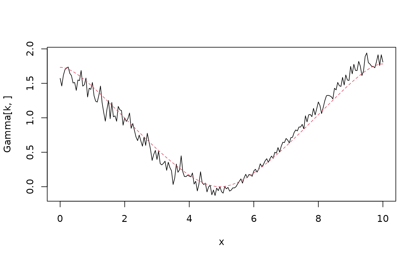
  # Compute and plot the variogram of the model
  Sigma <- op$A[,-1] %*% solve(op$Q[-1,-1], t(op$A[,-1]))
  One <- rep(1, times = ncol(Sigma))
  D <- diag(Sigma)
  Gamma <- 0.5 * (One %*% t(D) + D %*% t(One) - 2 * Sigma)
  k <- 100
  plot(x, Gamma[k, ], type = "l")
  lines(x,
    variogram.intrinsic.spde(x[k], x, kappa, alpha, beta, L = 10, d = 1),
    col = 2, lty = 2
  )
}