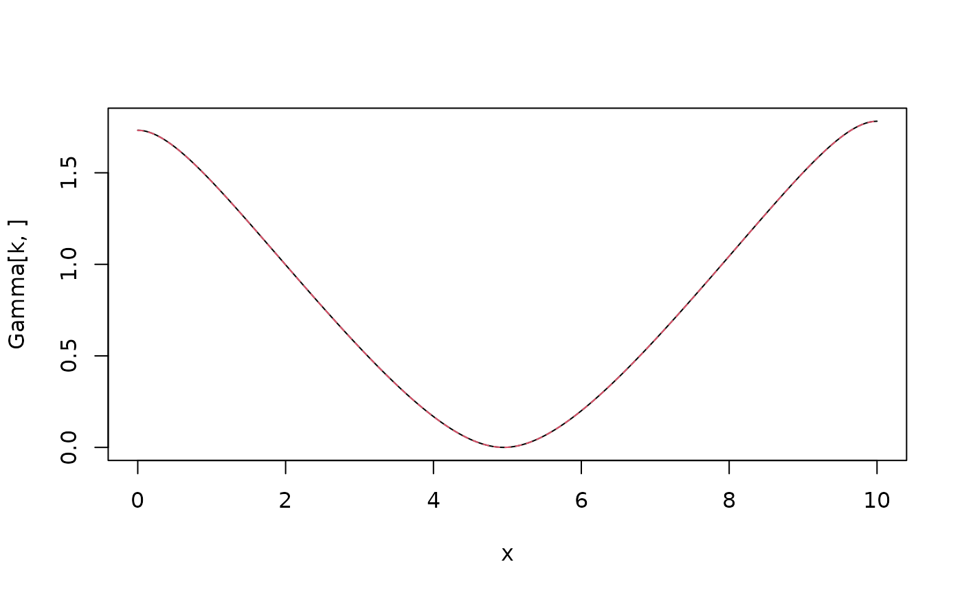
Variogram of intrinsic SPDE model

Variogram \(\gamma(s_0,s)\) of intrinsic SPDE model $$(-\Delta)^{\beta/2}(\kappa^2-\Delta)^{\alpha/2} (\tau u) = \mathcal{W}$$ with Neumann boundary conditions and a mean-zero constraint on a square \([0,L]^d\) for \(d=1\) or \(d=2\).

Usage

variogram.intrinsic.spde(
  s0 = NULL,
  s = NULL,
  kappa = NULL,
  alpha = NULL,
  beta = NULL,
  tau = 1,
  L = NULL,
  N = 100,
  d = NULL
)

Arguments

s0

The location where the variogram should be evaluated, either a double for 1d or a vector for 2d

s

A vector (in 1d) or matrix (in 2d) with all locations where the variogram is computed

kappa

Range parameter.

alpha

Smoothness parameter.

beta

Smoothness parameter.

tau

Precision parameter.

L

The side length of the square domain.

N

The number of terms in the Karhunen-Loeve expansion.

d

The dimension (1 or 2).

Details

The variogram is computed based on a Karhunen-Loeve expansion of the covariance function.

See also

intrinsic.matern.operators()

Examples

if (requireNamespace("RSpectra", quietly = TRUE)) {
  x <- seq(from = 0, to = 10, length.out = 201)
  beta <- 1
  alpha <- 1
  kappa <- 1
  op <- intrinsic.matern.operators(
    kappa = kappa, tau = 1, alpha = alpha,
    beta = beta, loc_mesh = x, d = 1
  )
  # Compute and plot the variogram of the model
  Sigma <- op$A %*% solve(op$Q, t(op$A))
  One <- rep(1, times = ncol(Sigma))
  D <- diag(Sigma)
  Gamma <- 0.5 * (One %*% t(D) + D %*% t(One) - 2 * Sigma)
  k <- 100
  plot(x, Gamma[k, ], type = "l")
  lines(x,
    variogram.intrinsic.spde(x[k], x, kappa, alpha, beta, L = 10, d = 1),
    col = 2, lty = 2
  )
}