Covariance-based approximations of intrinsic fields

intrinsic.matern.operators is used for computing a covariance-based rational SPDE approximation of intrinsic fields on \(R^d\) defined through the SPDE $$(-\Delta)^{\beta/2} (\tau u) = \mathcal{W}$$

Usage

intrinsic.operators(
  tau = NULL,
  beta = NULL,
  G = NULL,
  C = NULL,
  d = NULL,
  mesh = NULL,
  graph = NULL,
  loc_mesh = NULL,
  m = 1,
  compute_higher_order = FALSE,
  return_block_list = FALSE,
  type_rational_approximation = c("chebfun", "brasil", "chebfunLB"),
  fem_mesh_matrices = NULL,
  scaling = NULL,
  opts = NULL
)

Arguments

tau

precision parameter

beta

Smoothness parameter

G

The stiffness matrix of a finite element discretization of the domain of interest.

C

The mass matrix of a finite element discretization of the domain of interest.

d

The dimension of the domain.

mesh

An inla mesh.

graph

An optional metric_graph object. Replaces d, C and G.

loc_mesh

locations for the mesh for d=1.

m

The order of the rational approximation for the intrinsic part, which needs to be a positive integer. The default value is 2.

compute_higher_order

Logical. Should the higher order finite element matrices be computed?

return_block_list

Logical. For type = "covariance", should the block parts of the precision matrix be returned separately as a list?

type_rational_approximation

Which type of rational approximation should be used? The current types are "chebfun", "brasil" or "chebfunLB".

fem_mesh_matrices

A list containing FEM-related matrices. The list should contain elements c0, g1, g2, g3, etc.

scaling

scaling factor, see details.

opts

options for numerical calulcation of the scaling, see details.

Value

intrinsic.operators returns an object of class "intrinsicCBrSPDEobj".

Details

The covariance operator $$\tau^{-2}(-\Delta)^{\beta}$$ is approximated based on a rational approximation. The Laplacian is equipped with homogeneous Neumann boundary conditions and a zero-mean constraint is additionally imposed to obtained a non-intrinsic model. The scaling is computed as the lowest positive eigenvalue of sqrt(solve(c0))%*%g1sqrt(solve(c0)). opts provides a list of options for the numerical calculation of the scaling factor, which is done using Rspectra::eigs_sym. See the help of that function for details.

Examples

if (requireNamespace("RSpectra", quietly = TRUE)) {
  x <- seq(from = 0, to = 10, length.out = 201)
  beta <- 1
  alpha <- 1
  op <- intrinsic.operators(tau = 1, beta = beta, loc_mesh = x, d = 1)
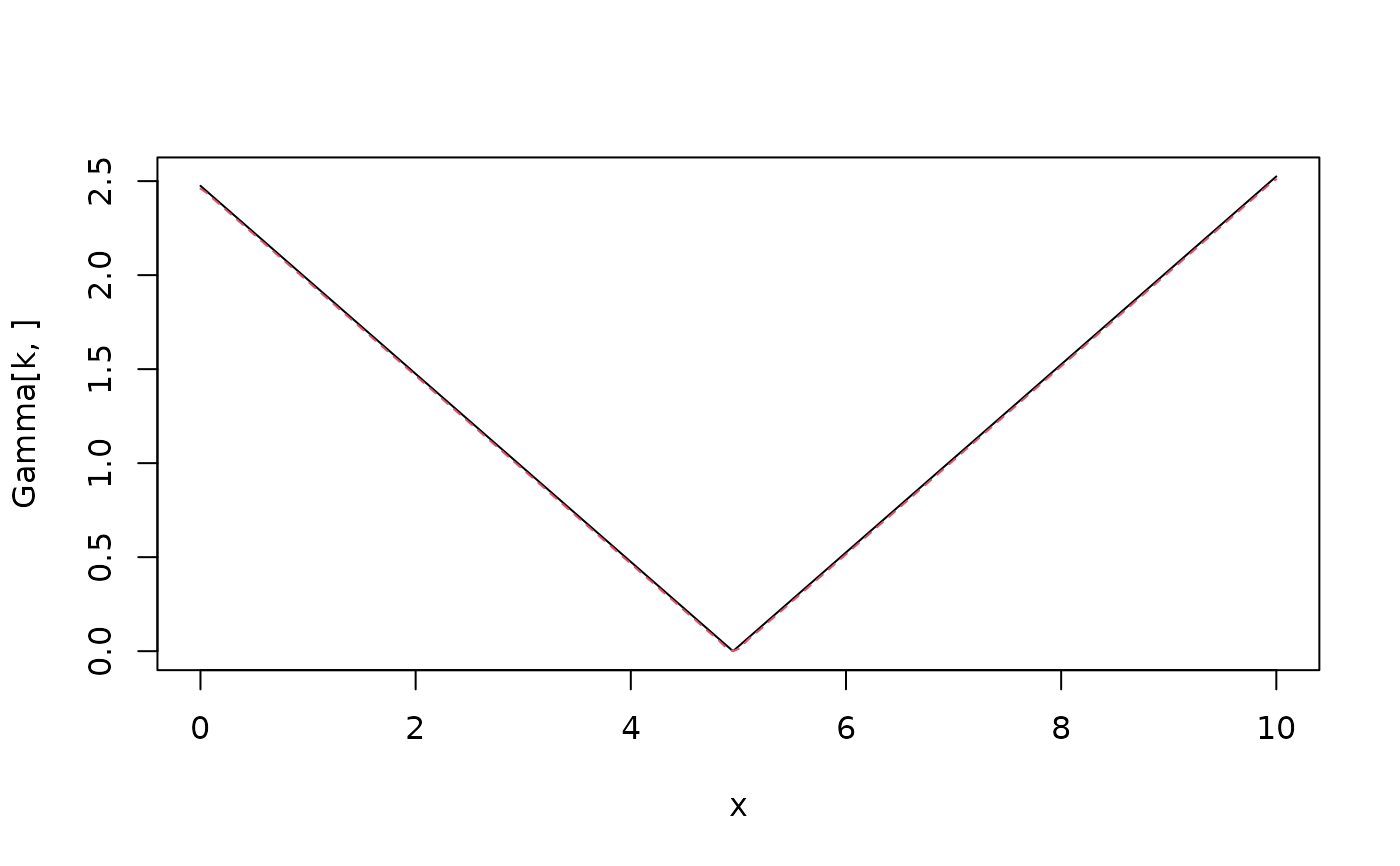
  # Compute and plot the variogram of the model
  Sigma <- op$A[,-1] %*% solve(op$Q[-1,-1], t(op$A[,-1]))
  One <- rep(1, times = ncol(Sigma))
  D <- diag(Sigma)
  Gamma <- 0.5 * (One %*% t(D) + D %*% t(One) - 2 * Sigma)
  k <- 100
  plot(x, Gamma[k, ], type = "l")
  lines(x,
    variogram.intrinsic.spde(x[k], x, kappa = 0, alpha = 0, 
    beta = beta, L = 10, d = 1),
    col = 2, lty = 2
  )
}