Prediction of a fractional SPDE using a rational SPDE approximation

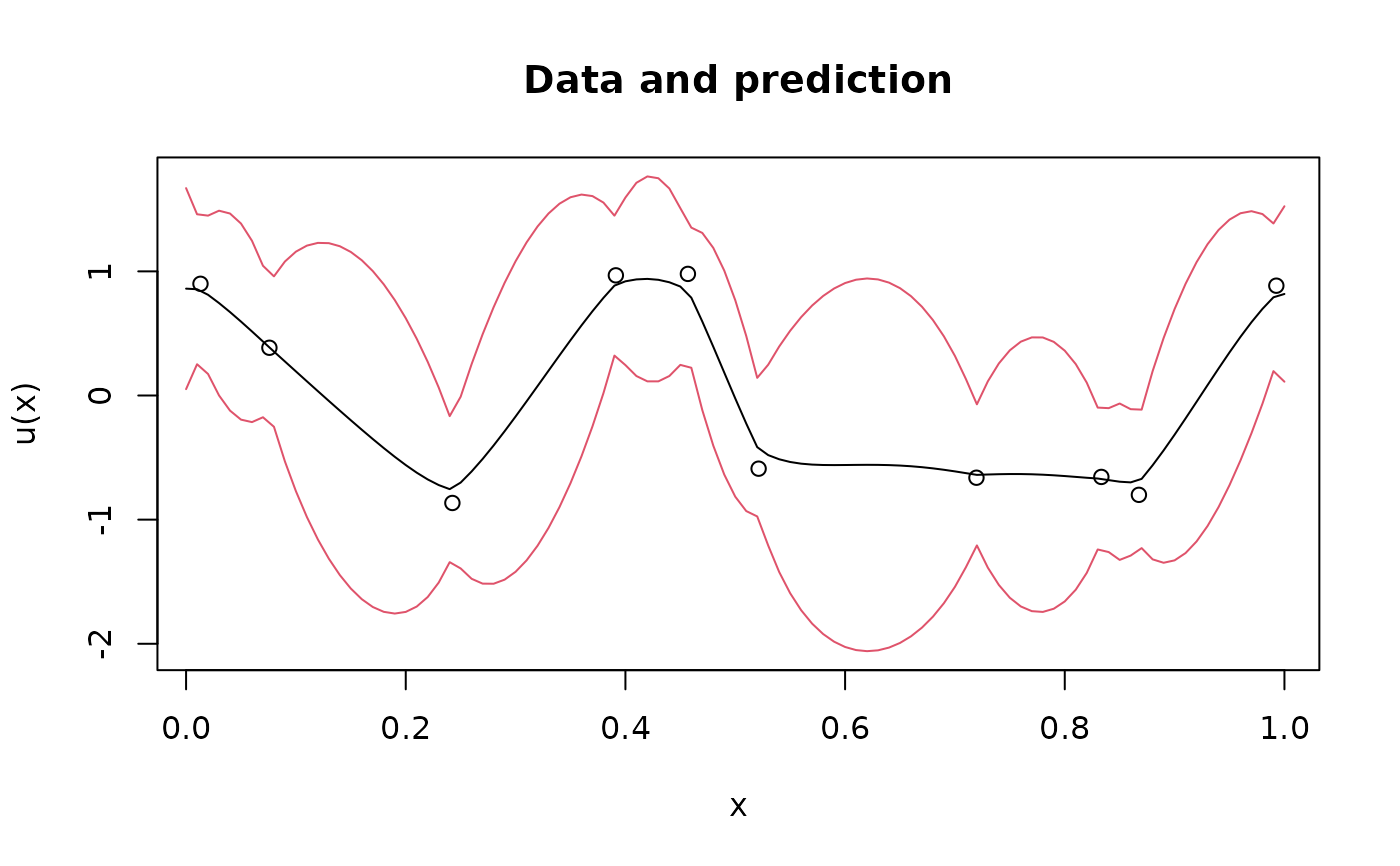
The function is used for computing kriging predictions based on data \(Y_i = u(s_i) + \epsilon_i\), where \(\epsilon\) is mean-zero Gaussian measurement noise and \(u(s)\) is defined by a fractional SPDE \(L^\beta u(s) = W\), where \(W\) is Gaussian white noise.

Usage

# S3 method for rSPDEobj
predict(
  object,
  A,
  Aprd,
  Y,
  sigma.e,
  compute.variances = FALSE,
  posterior_samples = FALSE,
  n_samples = 100,
  only_latent = FALSE,
  ...
)

Arguments

object

The rational SPDE approximation, computed using fractional.operators(), matern.operators(), or spde.matern.operators().

A

A matrix linking the measurement locations to the basis of the FEM approximation of the latent model.

Aprd

A matrix linking the prediction locations to the basis of the FEM approximation of the latent model.

Y

A vector with the observed data, can also be a matrix where the columns are observations of independent replicates of \(u\).

sigma.e

The standard deviation of the Gaussian measurement noise. Put to zero if the model does not have measurement noise.

compute.variances

Set to also TRUE to compute the kriging variances.

posterior_samples

If TRUE, posterior samples will be returned.

n_samples

Number of samples to be returned. Will only be used if sampling is TRUE.

only_latent

Should the posterior samples be only given to the latent model?

...

further arguments passed to or from other methods.

Value

A list with elements

mean

The kriging predictor (the posterior mean of u|Y).

variance

The posterior variances (if computed).

samples

A matrix containing the samples if sampling is TRUE.

Examples

# Sample a Gaussian Matern process on R using a rational approximation
kappa <- 10
sigma <- 1
nu <- 0.8
sigma.e <- 0.3
range <- sqrt(8 * nu) / kappa

# create mass and stiffness matrices for a FEM discretization
x <- seq(from = 0, to = 1, length.out = 101)
fem <- rSPDE.fem1d(x)

# compute rational approximation
op <- matern.operators(
  range = range, sigma = sigma,
  nu = nu, loc_mesh = x, d = 1,
  parameterization = "matern"
)

# Sample the model
u <- simulate(op)

# Create some data
obs.loc <- runif(n = 10, min = 0, max = 1)
A <- rSPDE.A1d(x, obs.loc)
Y <- as.vector(A %*% u + sigma.e * rnorm(10))

# compute kriging predictions at the FEM grid
A.krig <- rSPDE.A1d(x, x)
u.krig <- predict(op,
  A = A, Aprd = A.krig, Y = Y, sigma.e = sigma.e,
  compute.variances = TRUE
)

plot(obs.loc, Y,
  ylab = "u(x)", xlab = "x", main = "Data and prediction",
  ylim = c(
    min(u.krig$mean - 2 * sqrt(u.krig$variance)),
    max(u.krig$mean + 2 * sqrt(u.krig$variance))
  )
)
lines(x, u.krig$mean)
lines(x, u.krig$mean + 2 * sqrt(u.krig$variance), col = 2)
lines(x, u.krig$mean - 2 * sqrt(u.krig$variance), col = 2)