An introduction to the rSPDE package

Introduction

In this vignette we provide a brief introduction to the rSPDE package. The main approach for constructing the rational approximations is the covariance-based rational SPDE approach of Bolin, Simas, and Xiong (2023). The package contains three main “families” of functions that implement the approach:

an interface to R-INLA;
an interface to inlabru;
a stand-alone implementation of the approach.

To illustrate these different functions, we begin by using the package to generate a simple data set, which then will be analyzed using the different approaches. Further details on each family of functions is given in the following additional vignettes:

The rSPDE package also has a separate group of functions for performing the operator-based rational approximations introduced in Bolin and Kirchner (2020). These are especially useful when performing rational approximations for fractional SPDE models with non-Gaussian noise. An example in which such approximation is suitable is when one has the so-called type-G Lévy noises.

We refer the reader to Wallin and Bolin (2015), Bolin (2013) and Asar et al. (2020) for examples of models driven by type-G Lévy noises. We also refer the reader to the ngme package where one can fit such models.

We explore the functions for performing the operator-based rational approximation on the vignette:

Operator-based rational approximation with the rSPDE package

A toy data set

We begin by generating a toy data set.

For this illustration, we will simulate a data set on a two-dimensional spatial domain. To this end, we need to construct a mesh over the domain of interest and then compute the matrices needed to define the operator. We will use the R-INLA package to create the mesh and obtain the matrices of interest.

We will begin by defining a mesh over \([0,1]\times [0, 1]\):

library(fmesher)
n_loc <- 2000
loc_2d_mesh <- matrix(runif(n_loc * 2), n_loc, 2)
mesh_2d <- fm_mesh_2d(
  loc = loc_2d_mesh,
  cutoff = 0.05,
  max.edge = c(0.1, 0.5)
)
plot(mesh_2d, main = "")

We now use the matern.operators() function to construct a rational SPDE approximation of order \(m=2\) for a Gaussian random field with a Matérn covariance function on \([0,1]\times [0, 1]\). We choose \(\nu=0.5\) which corresponds to exponential covariance. We also set \(\sigma=1\) and the range as \(0.2\).

library(rSPDE)
sigma <- 2
range <- 0.25
nu <- 1.3
kappa <- sqrt(8 * nu) / range
op <- matern.operators(
  mesh = mesh_2d, nu = nu,
  range = range, sigma = sigma, m = 2,
  parameterization = "matern"
)
tau <- op$tau

We can now use the simulate function to simulate a realization of the field \(u\):

u <- simulate(op)

Let us now consider a simple Gaussian linear model where the spatial field \(u(\mathbf{s})\) is observed at \(m\) locations, \(\{\mathbf{s}_1 , \ldots , \mathbf{s}_m \}\) under Gaussian measurement noise. For each \(i = 1,\ldots,m,\) we have \[ \begin{align} y_i &= u(\mathbf{s}_i)+\varepsilon_i\\ \end{align}, \] where \(\varepsilon_1,\ldots,\varepsilon_{m}\) are iid normally distributed with mean 0 and standard deviation 0.1.

To generate a data set y from this model, we first draw some observation locations at random in the domain and then use the spde.make.A() functions (that wraps the functions fm_basis(), fm_block() and fm_row_kron() of the fmesher package) to construct the observation matrix which can be used to evaluate the simulated field \(u\) at the observation locations. After this we simply add the measurment noise.

A <- spde.make.A(
  mesh = mesh_2d,
  loc = loc_2d_mesh
)
sigma.e <- 0.1
y <- A %*% u + rnorm(n_loc) * sigma.e

The generated data can be seen in the following image.

library(ggplot2)
library(viridis)
#> Loading required package: viridisLite
df <- data.frame(x1 = as.double(loc_2d_mesh[, 1]),
  x2 = as.double(loc_2d_mesh[, 2]), y = as.double(y))
ggplot(df, aes(x = x1, y = x2, col = y)) +
  geom_point() +
  scale_color_viridis()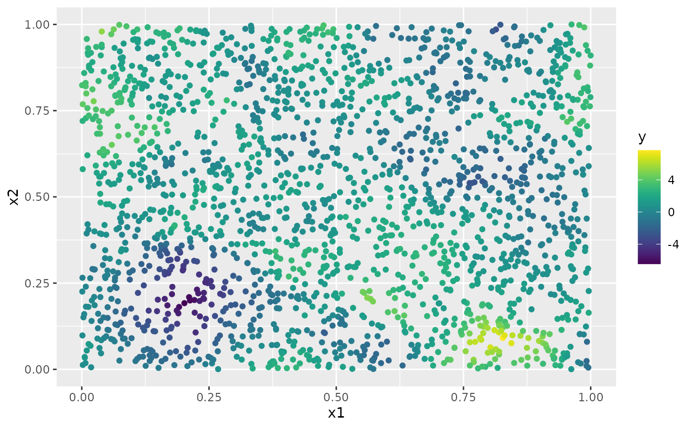

The simulated random field is shown in the following figure.

proj <- fm_evaluator(mesh_2d, dims = c(100, 100))
field <- fm_evaluate(proj, field = as.vector(u))
field.df <- data.frame(x1 = proj$lattice$loc[,1],
                        x2 = proj$lattice$loc[,2], 
                        y = as.vector(field))
ggplot(field.df, aes(x = x1, y = x2, fill = y)) +
  geom_raster() + xlim(0,1) + ylim(0,1) + 
  scale_fill_viridis()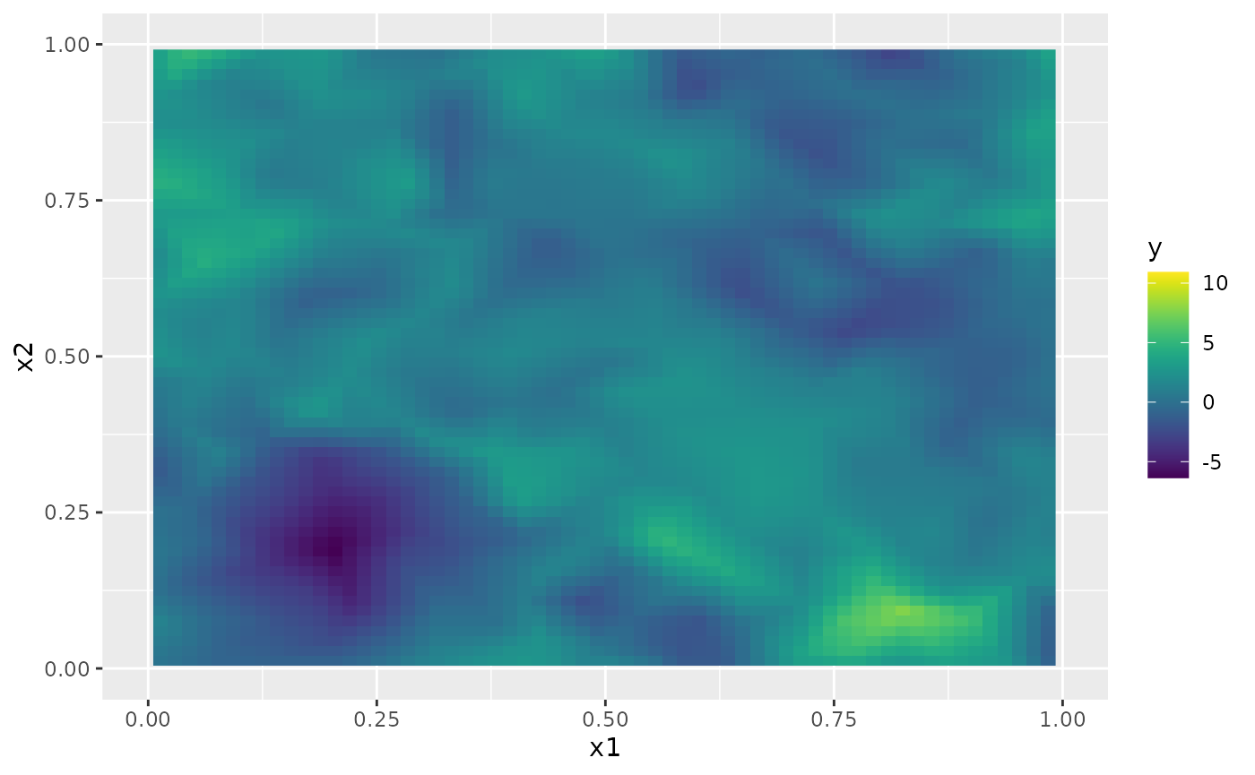

Fitting the model with `R-INLA` implementation of the rational SPDE approach

We will now fit the model of the toy data set using our R-INLA implementation of the rational SPDE approach. Further details on this implementation can be found in R-INLA implementation of the rational SPDE approach.

We begin by loading the INLA package and creating the \(A\) matrix, the index, and the inla.stack object.

library(INLA)
#> Loading required package: sp
#> This is INLA_24.04.01 built 2024-04-01 19:43:22 UTC.
#>  - See www.r-inla.org/contact-us for how to get help.
#>  - List available models/likelihoods/etc with inla.list.models()
#>  - Use inla.doc(<NAME>) to access documentation

Abar <- rspde.make.A(mesh = mesh_2d, loc = loc_2d_mesh)
mesh.index <- rspde.make.index(name = "field", mesh = mesh_2d)

st.dat <- inla.stack(
  data = list(y = as.vector(y)),
  A = Abar,
  effects = mesh.index
)

We now create the model object. We need to set an upper bound for the smoothness parameter \(\nu\). The default value for this is \(4\). If we increase the upper bound for \(\nu\) we also increase the computational cost, and if we decrease the upper bound we also decrease the computatoinal cost. For this example we set nu.upper.bound=2. See the R-INLA implementation of the rational SPDE approach for further details.

rspde_model <- rspde.matern(
  mesh = mesh_2d,
  nu.upper.bound = 2,
  parameterization = "spde"
)

Finally, we create the formula and fit the model to the data:

f <-
  y ~ -1 + f(field, model = rspde_model)
rspde_fit <-
  inla(f,
    data = inla.stack.data(st.dat),
    family = "gaussian",
    control.predictor =
      list(A = inla.stack.A(st.dat))
  )

We can get a summary of the fit:

summary(rspde_fit)
#> Time used:
#>     Pre = 0.412, Running = 2.49, Post = 0.144, Total = 3.05 
#> Random effects:
#>   Name     Model
#>     field CGeneric
#> 
#> Model hyperparameters:
#>                                            mean    sd 0.025quant 0.5quant
#> Precision for the Gaussian observations 101.668 3.497     94.925  101.618
#> Theta1 for field                         -3.684 0.123     -3.935   -3.681
#> Theta2 for field                          2.171 0.142      1.886    2.173
#> Theta3 for field                         -0.373 0.079     -0.521   -0.376
#>                                         0.975quant    mode
#> Precision for the Gaussian observations    108.693 101.543
#> Theta1 for field                            -3.451  -3.668
#> Theta2 for field                             2.445   2.182
#> Theta3 for field                            -0.211  -0.386
#> 
#> Marginal log-Likelihood:  853.65 
#>  is computed 
#> Posterior summaries for the linear predictor and the fitted values are computed
#> (Posterior marginals needs also 'control.compute=list(return.marginals.predictor=TRUE)')

To get a summary of the fit of the random field only, we can do the following:

result_fit <- rspde.result(rspde_fit, "field", rspde_model)
summary(result_fit)
#>            mean         sd 0.025quant  0.5quant 0.975quant     mode
#> tau   0.0253177 0.00308018  0.0196175 0.0252343  0.0316572 0.025131
#> kappa 8.8568800 1.24979000  6.6087000 8.7904300 11.5069000 8.678790
#> nu    0.8157250 0.03785310  0.7456920 0.8140100  0.8940130 0.808801
tau <- op$tau
result_df <- data.frame(
  parameter = c("tau", "kappa", "nu"),
  true = c(tau, kappa, nu), mean = c(
    result_fit$summary.tau$mean,
    result_fit$summary.kappa$mean,
    result_fit$summary.nu$mean
  ),
  mode = c(
    result_fit$summary.tau$mode,
    result_fit$summary.kappa$mode,
    result_fit$summary.nu$mode
  )
)
print(result_df)
#>   parameter         true       mean       mode
#> 1       tau  0.004452908 0.02531772 0.02513105
#> 2     kappa 12.899612397 8.85688316 8.67878895
#> 3        nu  1.300000000 0.81572477 0.80880095

We can also obtain the summary in the matern parameterization by setting the parameterization argument to matern:

result_fit_matern <- rspde.result(rspde_fit, "field", rspde_model,
                                  parameterization = "matern")
summary(result_fit_matern)
#>             mean        sd 0.025quant 0.5quant 0.975quant     mode
#> std.dev 2.667680 0.3017070   2.155940 2.638550   3.327100 2.601860
#> range   0.296234 0.0456056   0.217838 0.292395   0.395099 0.288219
#> nu      0.815725 0.0378531   0.745692 0.814010   0.894013 0.808801
result_df_matern <- data.frame(
  parameter = c("sigma", "range", "nu"),
  true = c(sigma, range, nu), mean = c(
    result_fit_matern$summary.std.dev$mean,
    result_fit_matern$summary.range$mean,
    result_fit_matern$summary.nu$mean
  ),
  mode = c(
    result_fit_matern$summary.std.dev$mode,
    result_fit_matern$summary.range$mode,
    result_fit_matern$summary.nu$mode
  )
)
print(result_df_matern)
#>   parameter true      mean      mode
#> 1     sigma 2.00 2.6676797 2.6018639
#> 2     range 0.25 0.2962344 0.2882185
#> 3        nu 1.30 0.8157248 0.8088009

Kriging with `R-INLA` implementation of the rational SPDE approach

Let us now obtain predictions (i.e., do kriging) of the latent field on a dense grid in the region.

We begin by creating the grid of locations where we want to compute the predictions. To this end, we can use the rspde.mesh.projector() function. This function has the same arguments as the function inla.mesh.projector() the only difference being that the rSPDE version also has an argument nu and an argument rspde.order. Thus, we proceed in the same fashion as we would in R-INLA’s standard SPDE implementation:

projgrid <- rspde.mesh.projector(mesh_2d,
  xlim = c(0, 1),
  ylim = c(0, 1)
)

This lattice contains 100 × 100 locations (the default) which are shown in the following figure:

coord.prd <- projgrid$lattice$loc
plot(coord.prd, type = "p", cex = 0.1)

Let us now calculate the predictions jointly with the estimation. To this end, first, we begin by linking the prediction coordinates to the mesh nodes through an \(A\) matrix

A.prd <- projgrid$proj$A

We now make a stack for the prediction locations. We have no data at the prediction locations, so we set y= NA. We then join this stack with the estimation stack.

ef.prd <- list(c(mesh.index))
st.prd <- inla.stack(
  data = list(y = NA),
  A = list(A.prd), tag = "prd",
  effects = ef.prd
)
st.all <- inla.stack(st.dat, st.prd)

Doing the joint estimation takes a while, and we therefore turn off the computation of certain things that we are not interested in, such as the marginals for the random effect. We will also use a simplified integration strategy (actually only using the posterior mode of the hyper-parameters) through the command control.inla = list(int.strategy = "eb"), i.e. empirical Bayes:

rspde_fitprd <- inla(f,
  family = "Gaussian",
  data = inla.stack.data(st.all),
  control.predictor = list(
    A = inla.stack.A(st.all),
    compute = TRUE, link = 1
  ),
  control.compute = list(
    return.marginals = FALSE,
    return.marginals.predictor = FALSE
  ),
  control.inla = list(int.strategy = "eb")
)

We then extract the indices to the prediction nodes and then extract the mean and the standard deviation of the response:

id.prd <- inla.stack.index(st.all, "prd")$data
m.prd <- matrix(rspde_fitprd$summary.fitted.values$mean[id.prd], 100, 100)
sd.prd <- matrix(rspde_fitprd$summary.fitted.values$sd[id.prd], 100, 100)

Finally, we plot the results. First the mean:

field.pred.df <- data.frame(x1 = projgrid$lattice$loc[,1],
                        x2 = projgrid$lattice$loc[,2], 
                        y = as.vector(m.prd))
ggplot(field.pred.df, aes(x = x1, y = x2, fill = y)) +
  geom_raster() + xlim(0,1) + ylim(0,1) + 
  scale_fill_viridis()
#> Warning: Removed 396 rows containing missing values or values outside the scale range
#> (`geom_raster()`).

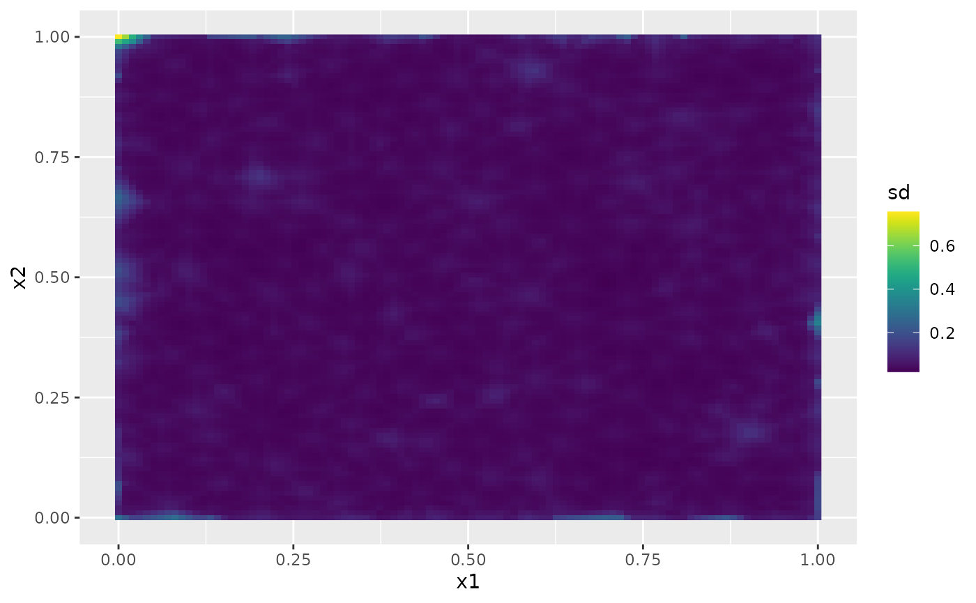
Then, the marginal standard deviations:

field.pred.sd.df <- data.frame(x1 = proj$lattice$loc[,1],
                        x2 = proj$lattice$loc[,2], 
                        sd = as.vector(sd.prd))
ggplot(field.pred.sd.df, aes(x = x1, y = x2, fill = sd)) +
  geom_raster() + xlim(0,1) + ylim(0,1) + 
  geom_raster() +
  scale_fill_viridis()
#> Warning: Removed 6156 rows containing missing values or values outside the scale range
#> (`geom_raster()`).
#> Removed 6156 rows containing missing values or values outside the scale range
#> (`geom_raster()`).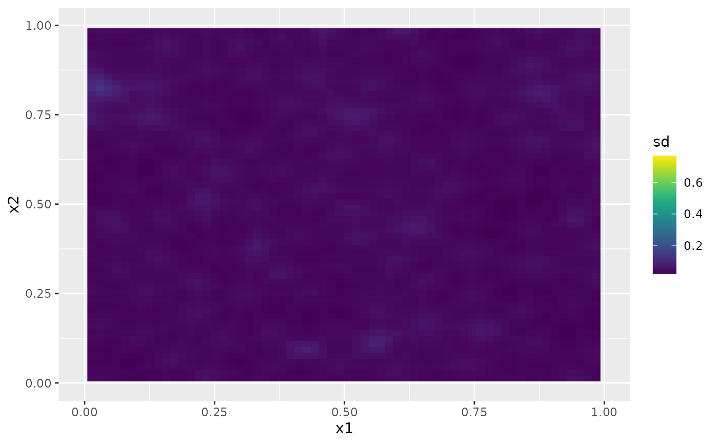

Fitting the model with `inlabru` implementation of the rational SPDE approach

We will now fit the same model of the toy data set using our inlabru implementation of the rational SPDE approach. Further details on this implementation can be found in inlabru implementation of the rational SPDE approach.

We begin by loading the inlabru package:

library(inlabru)

The creation of the model object is the same as in R-INLA’s case:

rspde_model <- rspde.matern(
  mesh = mesh_2d,
  nu.upper.bound = 2,
  parameterization = "spde"
)

The advantage with inlabru is that we do not need to form the stack manually, but can simply collect the required data in a data.frame():

toy_df <- data.frame(coord1 = loc_2d_mesh[,1],
                     coord2 = loc_2d_mesh[,2],
                     y = as.vector(y))
coordinates(toy_df) <- c("coord1", "coord2")

Finally, we create the component and fit:

cmp <-
  y ~ -1 + field(coordinates, model = rspde_model)

rspde_bru_fit <-
  bru(cmp,
      data=toy_df,
    options=list(
    family = "gaussian")
  )

At this stage, we can get a summary of the fit just as in the R-INLA case:

summary(rspde_bru_fit)
#> inlabru version: 2.10.1
#> INLA version: 24.04.01
#> Components:
#> field: main = cgeneric(coordinates), group = exchangeable(1L), replicate = iid(1L)
#> Likelihoods:
#>   Family: 'gaussian'
#>     Data class: 'SpatialPointsDataFrame'
#>     Predictor: y ~ .
#> Time used:
#>     Pre = 0.177, Running = 2.57, Post = 0.451, Total = 3.2 
#> Random effects:
#>   Name     Model
#>     field CGeneric
#> 
#> Model hyperparameters:
#>                                            mean    sd 0.025quant 0.5quant
#> Precision for the Gaussian observations 101.668 3.497     94.925  101.618
#> Theta1 for field                         -3.684 0.123     -3.935   -3.681
#> Theta2 for field                          2.171 0.142      1.886    2.173
#> Theta3 for field                         -0.373 0.079     -0.521   -0.376
#>                                         0.975quant    mode
#> Precision for the Gaussian observations    108.693 101.543
#> Theta1 for field                            -3.451  -3.668
#> Theta2 for field                             2.445   2.182
#> Theta3 for field                            -0.211  -0.386
#> 
#> Deviance Information Criterion (DIC) ...............: -3266.47
#> Deviance Information Criterion (DIC, saturated) ....: 2300.60
#> Effective number of parameters .....................: 297.95
#> 
#> Watanabe-Akaike information criterion (WAIC) ...: -3257.99
#> Effective number of parameters .................: 265.51
#> 
#> Marginal log-Likelihood:  853.65 
#>  is computed 
#> Posterior summaries for the linear predictor and the fitted values are computed
#> (Posterior marginals needs also 'control.compute=list(return.marginals.predictor=TRUE)')

and also obtain a summary of the field only:

result_fit <- rspde.result(rspde_bru_fit, "field", rspde_model)
summary(result_fit)
#>            mean         sd 0.025quant  0.5quant 0.975quant      mode
#> tau   0.0253177 0.00308019  0.0196175 0.0252343  0.0316572 0.0251311
#> kappa 8.8569000 1.24979000  6.6087200 8.7904400 11.5069000 8.6788000
#> nu    0.8157250 0.03785310  0.7456920 0.8140100  0.8940120 0.8088010
tau <- op$tau
result_df <- data.frame(
  parameter = c("tau", "kappa", "nu"),
  true = c(tau, kappa, nu), mean = c(
    result_fit$summary.tau$mean,
    result_fit$summary.kappa$mean,
    result_fit$summary.nu$mean
  ),
  mode = c(
    result_fit$summary.tau$mode,
    result_fit$summary.kappa$mode,
    result_fit$summary.nu$mode
  )
)
print(result_df)
#>   parameter         true       mean       mode
#> 1       tau  0.004452908 0.02531772 0.02513105
#> 2     kappa 12.899612397 8.85689539 8.67879856
#> 3        nu  1.300000000 0.81572455 0.80880077

Let us obtain a summary in the matern parameterization by setting the parameterization argument to matern:

result_fit_matern <- rspde.result(rspde_bru_fit, "field", rspde_model,
                                  parameterization = "matern")
summary(result_fit_matern)
#>             mean        sd 0.025quant 0.5quant 0.975quant     mode
#> std.dev 2.668300 0.2969180   2.166850 2.640250   3.322540 2.625630
#> range   0.296292 0.0450992   0.219145 0.292483   0.394673 0.285176
#> nu      0.815725 0.0378531   0.745692 0.814010   0.894012 0.808801
result_df_matern <- data.frame(
  parameter = c("sigma", "range", "nu"),
  true = c(sigma, range, nu), mean = c(
    result_fit_matern$summary.std.dev$mean,
    result_fit_matern$summary.range$mean,
    result_fit_matern$summary.nu$mean
  ),
  mode = c(
    result_fit_matern$summary.std.dev$mode,
    result_fit_matern$summary.range$mode,
    result_fit_matern$summary.nu$mode
  )
)
print(result_df_matern)
#>   parameter true      mean      mode
#> 1     sigma 2.00 2.6683017 2.6256324
#> 2     range 0.25 0.2962918 0.2851756
#> 3        nu 1.30 0.8157246 0.8088008

Kriging with `inlabru` implementation of the rational SPDE approach

Let us now obtain predictions (i.e., do kriging) of the latent field on a dense grid in the region.

We begin by creating the grid of the locations where we want to evaluate the predictions. We begin by creating a regular grid in and then extract the coorinates:

pred_coords <- data.frame(x1 = projgrid$lattice$loc[,1],
                          x2 = projgrid$lattice$loc[,2])
coordinates(pred_coords) <- c("x1", "x2")

Let us now compute the predictions. An advantage with inlabru is that we can do this after fitting the model to the data:

field_pred <- predict(rspde_bru_fit, pred_coords, ~field)

The following figure shows the mean of these predictions:

field_pred_df <- field_pred@data
field_pred_df <- cbind(field_pred_df, field_pred@coords)
ggplot(field_pred_df, aes(x = x1, y = x2, fill = mean)) +
  geom_raster() + xlim(0,1) + ylim(0,1) + 
  scale_fill_viridis()

The following figure shows the marginal standard deviations of the predictions:

ggplot(field_pred_df, aes(x = x1, y = x2, fill = sd)) +
  geom_raster() + xlim(0,1) + ylim(0,1) + 
  scale_fill_viridis()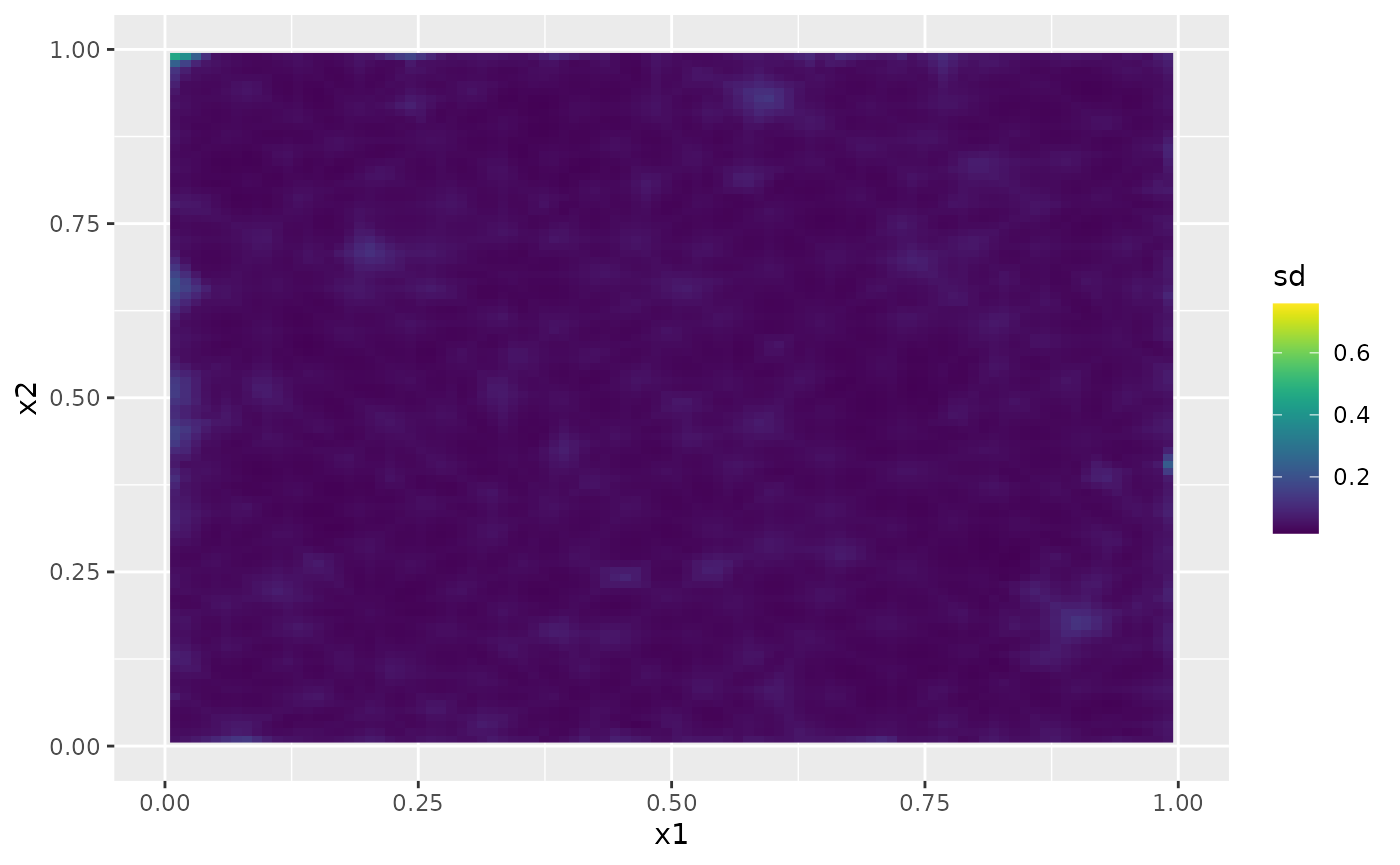

An alternative and very simple approach is to use the pixels() function:

pxl <- pixels(mesh_2d)

field_pred <- predict(rspde_bru_fit, pxl, ~field)

ggplot() + gg(field_pred) +
  scale_fill_viridis() + xlim(0,1) + ylim(0,1)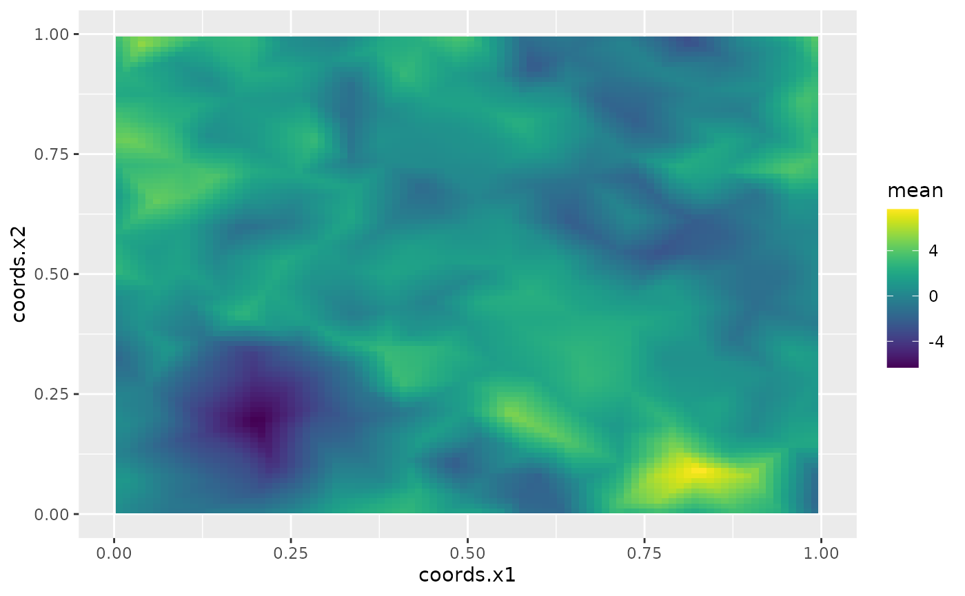

Fitting the model with `rSPDE`

We will now fit the model of the toy data set without using R-INLA or inlabru. To this end we will use the rational approximation functions from rSPDE package. Further details can be found in the vignette Rational approximation with the rSPDE package.

We use the function rSPDE.construct.matern.loglike() to define the likelihood. This function is object-based, in the sense that it obtains several of the quantities it needs from the rSPDE model object.

Notice that we already created a rSPDE model object to simulate the data. We will, then, use the same model object. Recall that the rSPDE model object we created is op.

Let us create an object for estimation, a data.frame with the data and then fit the model using the rspde_lme() function.

op_est <- matern.operators(
  mesh = mesh_2d, m = 2
)

toy_df_rspde <- data.frame(coord1 = loc_2d_mesh[,1],
                     coord2 = loc_2d_mesh[,2],
                     y = as.vector(y))

fit_rspde <- rspde_lme(y ~ -1, data = toy_df_rspde, loc = c("coord1", "coord2"),
                      model = op_est, parallel = TRUE)

We can obtain the summary:

summary(fit_rspde)
#> 
#> Latent model - Whittle-Matern
#> 
#> Call:
#> rspde_lme(formula = y ~ -1, loc = c("coord1", "coord2"), data = toy_df_rspde, 
#>     model = op_est, parallel = TRUE)
#> 
#> No fixed effects.
#> 
#> Random effects:
#>        Estimate Std.error z-value
#> alpha 2.342e+00 2.826e-02  82.856
#> tau   3.498e-03 4.279e-04   8.176
#> kappa 1.412e+01 1.462e+00   9.659
#> 
#> Random effects (Matern parameterization):
#>       Estimate Std.error z-value
#> nu     1.34192   0.02826   47.48
#> sigma  1.99425   0.17988   11.09
#> range  0.23209   0.02380    9.75
#> 
#> Measurement error:
#>          Estimate Std.error z-value
#> std. dev 0.099239  0.001701   58.33
#> ---
#> Signif. codes:  0 '***' 0.001 '**' 0.01 '*' 0.05 '.' 0.1 ' ' 1 
#> 
#> Log-Likelihood:  871.6474 
#> Number of function calls by 'optim' = 86
#> Optimization method used in 'optim' = L-BFGS-B
#> 
#> Time used to:     fit the model =  15.75603 secs 
#>   set up the parallelization = 4.01611 secs

Let us compare with the true values:

print(data.frame(
  sigma = c(sigma, fit_rspde$matern_coeff$random_effects[2]), 
  range = c(range, fit_rspde$matern_coeff$random_effects[3]),
  nu = c(nu, fit_rspde$matern_coeff$random_effects[1]),
  row.names = c("Truth", "Estimates")
))
#>              sigma    range       nu
#> Truth     2.000000 0.250000 1.300000
#> Estimates 1.994253 0.232088 1.341924

# Time to fit
print(fit_rspde$fitting_tim)
#> Time difference of 15.75604 secs

Kriging with `rSPDE`

We will now do kriging on the same dense grid we did for the R-INLA-based rational SPDE approach, but now using the rSPDE functions. To this end we will use the predict method on the rSPDE model object.

Observe that we need an \(A\) matrix connecting the mesh to the prediction locations.

Let us now create the data.frame with the prediction locations:

predgrid <- fm_evaluator(mesh_2d,
  xlim = c(0, 1),
  ylim = c(0, 1)
)
pred_coords <- data.frame(coord1 = predgrid$lattice$loc[,1],
                          coord2 = predgrid$lattice$loc[,2])

We will now use the predict() method on the rSPDE model object with the argument compute.variances set to TRUE so that we can plot the standard deviations. Let us also update the values of the rSPDE model object to the fitted ones, and also save the estimated value of sigma.e.

pred.rspde <- predict(fit_rspde,
  data = pred_coords, loc = c("coord1", "coord2"),
  compute_variances = TRUE
)
#> Warning: The `data` argument of `predict()` is deprecated as of rSPDE 2.3.3.
#> ℹ Please use the `newdata` argument instead.
#> ℹ `data` was provided but not `newdata`. Setting `newdata <- data`.
#> This warning is displayed once every 8 hours.
#> Call `lifecycle::last_lifecycle_warnings()` to see where this warning was
#> generated.

Finally, we plot the results. First the mean:

field.pred2.df <- data.frame(x1 = predgrid$lattice$loc[,1],
                             x2 = predgrid$lattice$loc[,2],
                             y = as.vector(pred.rspde$mean))
ggplot(field.pred2.df, aes(x = x1, y = x2, fill = y)) +
  geom_raster() + xlim(0,1) + ylim(0,1) + 
  scale_fill_viridis()
#> Warning: Removed 396 rows containing missing values or values outside the scale range
#> (`geom_raster()`).

Then, the standard deviations:

field.pred2.sd.df <-field.pred2.df <- data.frame(x1 = predgrid$lattice$loc[,1],
                             x2 = predgrid$lattice$loc[,2],
                             sd = as.vector(sqrt(pred.rspde$variance)))
ggplot(field.pred2.sd.df, aes(x = x1, y = x2, fill = sd)) +
  geom_raster() +
  scale_fill_viridis()

References

Asar, Özgür, David Bolin, Peter Diggle, and Jonas Wallin. 2020. “Linear Mixed Effects Models for Non‐Gaussian Repeated Measurement Data.” Journal of the Royal Statistical Society. Series C. Applied Statistics 69 (5): 1015–65.

Bolin, David. 2013. “Spatial Matérn Fields Driven by Non-Gaussian Noise.” Scandinavian Journal of Statistics 41 (3): 557–79.

Bolin, David, and Kristin Kirchner. 2020. “The Rational SPDE Approach for Gaussian Random Fields with General Smoothness.” Journal of Computational and Graphical Statistics 29 (2): 274–85.

Bolin, David, Alexandre B. Simas, and Zhen Xiong. 2023. “Covariance-Based Rational Approximations of Fractional SPDEs for Computationally Efficient Bayesian Inference.” Journal of Computational and Graphical Statistics.

Wallin, Jonas, and David Bolin. 2015. “Geostatistical Modelling Using Non-Gaussian Matérn Fields.” Scandinavian Journal of Statistics 42 (3): 872–90.

David Bolin and Alexandre B. Simas

2024-04-01

Introduction

A toy data set

Fitting the model with R-INLA implementation of the rational SPDE approach

Kriging with R-INLA implementation of the rational SPDE approach

Fitting the model with inlabru implementation of the rational SPDE approach

Kriging with inlabru implementation of the rational SPDE approach

Fitting the model with rSPDE