Comparison of different models using real data

David Bolin, Alexandre B. Simas, and Jonas Wallin

Created: 2024-02-09. Last modified: 2024-05-08.

Introduction

This vignette contains the details of the Application section of Bolin, Simas, and Wallin (2023). Our goal is to compare the predictive power of different models on metric graphs by cross-validation. More precisely, we consider the Whittle–Matérn fields introduced by Bolin, Simas, and Wallin (2024) and Bolin, Simas, and Wallin (2023), a Gaussian random field with an isotropic exponential covariance function Anderes, Møller, and Rasmussen (2020), and Matérn Gaussian processes based on the graph Laplacian Borovitskiy et al. (2021).

The dataset

For this example we will consider the pems data contained in the MetricGraph package. The data consists of traffic speed observations on highways in the city of San Jose, California. The variable y contains the traffic speeds.

 pems_graph <- metric_graph$new(edges = pems$edges, longlat=TRUE)
 pems_graph$add_observations(data = pems$data, normalized=TRUE)

Let us take a look at the observations:

pems_graph$plot(data = "y", vertex_size = 0)

The models

We will assume that the data has the following structure:

\[ y_i = \mu + u(s_i) + \varepsilon_i, \quad i=1,\ldots,n, \] where \(\mu\) is a constant that represents the mean of the field, \(u(\cdot)\) is a Gaussian random field, \(s_i\in \Gamma\) are observation locations and \(\varepsilon_i\) are independent centered Gaussian variables \(N(0,\sigma_e^2)\) representing measurement noise.

Let us fit the different models, that is, we will assume several different possible latent fields \(u(\cdot)\). We start by fitting a Whittle-Matérn field with alpha = 1:

fit_alpha1 <- graph_lme(y ~ 1, graph=pems_graph, 
            model = list(type = "WhittleMatern", alpha = 1))

and look at its summary:

summary(fit_alpha1)
#> 
#> Latent model - Whittle-Matern with alpha = 1
#> 
#> Call:
#> graph_lme(formula = y ~ 1, graph = pems_graph, model = list(type = "WhittleMatern", 
#>     alpha = 1))
#> 
#> Fixed effects:
#>             Estimate Std.error z-value Pr(>|z|)    
#> (Intercept)   51.205     4.114   12.45   <2e-16 ***
#> 
#> Random effects:
#>       Estimate Std.error z-value
#> tau   0.104439  0.007826  13.345
#> kappa 0.108664  0.049911   2.177
#> 
#> Random effects (Matern parameterization):
#>       Estimate Std.error z-value
#> sigma   20.539     4.358   4.713
#> range   18.405     8.438   2.181
#> 
#> Measurement error:
#>          Estimate Std.error z-value
#> std. dev   6.8629    0.4084   16.81
#> ---
#> Signif. codes:  0 '***' 0.001 '**' 0.01 '*' 0.05 '.' 0.1 ' ' 1 
#> 
#> Log-Likelihood:  -1221.225 
#> Number of function calls by 'optim' = 28
#> Optimization method used in 'optim' = L-BFGS-B
#> 
#> Time used to:     fit the model =  29.66951 secs

Now, we will fit a Whittle-Matérn field with alpha = 2:

fit_alpha2 <- graph_lme(y ~ 1, graph=pems_graph, 
            model = list(type = "WhittleMatern", alpha = 2))

and its summary:

summary(fit_alpha2)
#> 
#> Latent model - Whittle-Matern with alpha = 2
#> 
#> Call:
#> graph_lme(formula = y ~ 1, graph = pems_graph, model = list(type = "WhittleMatern", 
#>     alpha = 2))
#> 
#> Fixed effects:
#>             Estimate Std.error z-value Pr(>|z|)    
#> (Intercept)   51.164     2.797   18.29   <2e-16 ***
#> 
#> Random effects:
#>       Estimate Std.error z-value
#> tau    0.08662   0.01553   5.579
#> kappa  0.44612   0.07523   5.930
#> 
#> Random effects (Matern parameterization):
#>       Estimate Std.error z-value
#> sigma   19.372     2.532   7.651
#> range    7.765     1.281   6.063
#> 
#> Measurement error:
#>          Estimate Std.error z-value
#> std. dev   7.2348    0.3721   19.44
#> ---
#> Signif. codes:  0 '***' 0.001 '**' 0.01 '*' 0.05 '.' 0.1 ' ' 1 
#> 
#> Log-Likelihood:  -1207.996 
#> Number of function calls by 'optim' = 29
#> Optimization method used in 'optim' = L-BFGS-B
#> 
#> Time used to:     fit the model =  50.60577 secs

We will now fit Whittle-Matérn fields with alpha = 1 and alpha=2, and by performing a boundary correction on vertices of degree 1. To such an end, we set BC=1:

fit_alpha1_bc <- graph_lme(y ~ 1, graph=pems_graph, BC = 1,
        model = list(type = "WhittleMatern", alpha = 1))

fit_alpha2_bc <- graph_lme(y ~ 1, graph=pems_graph, BC = 1,
        model = list(type = "WhittleMatern", alpha = 2))

Now, let us look at the summaries:

summary(fit_alpha1_bc)
#> 
#> Latent model - Whittle-Matern with alpha = 1
#> 
#> Call:
#> graph_lme(formula = y ~ 1, graph = pems_graph, model = list(type = "WhittleMatern", 
#>     alpha = 1), BC = 1)
#> 
#> Fixed effects:
#>             Estimate Std.error z-value Pr(>|z|)    
#> (Intercept)   51.157     4.289   11.93   <2e-16 ***
#> 
#> Random effects:
#>       Estimate Std.error z-value
#> tau   0.104589  0.007829   13.36
#> kappa 0.095231  0.051193    1.86
#> 
#> Random effects (Matern parameterization):
#>       Estimate Std.error z-value
#> sigma   21.908     5.474   4.002
#> range   21.002    11.268   1.864
#> 
#> Measurement error:
#>          Estimate Std.error z-value
#> std. dev   6.8638    0.4083   16.81
#> ---
#> Signif. codes:  0 '***' 0.001 '**' 0.01 '*' 0.05 '.' 0.1 ' ' 1 
#> 
#> Log-Likelihood:  -1221.377 
#> Number of function calls by 'optim' = 32
#> Optimization method used in 'optim' = L-BFGS-B
#> 
#> Time used to:     fit the model =  34.91937 secs

and

summary(fit_alpha2_bc)
#> 
#> Latent model - Whittle-Matern with alpha = 2
#> 
#> Call:
#> graph_lme(formula = y ~ 1, graph = pems_graph, model = list(type = "WhittleMatern", 
#>     alpha = 2), BC = 1)
#> 
#> Fixed effects:
#>             Estimate Std.error z-value Pr(>|z|)    
#> (Intercept)   51.119     2.822   18.11   <2e-16 ***
#> 
#> Random effects:
#>       Estimate Std.error z-value
#> tau    0.08749   0.01566   5.586
#> kappa  0.43350   0.07515   5.768
#> 
#> Random effects (Matern parameterization):
#>       Estimate Std.error z-value
#> sigma   20.022     2.731   7.331
#> range    7.991     1.355   5.895
#> 
#> Measurement error:
#>          Estimate Std.error z-value
#> std. dev   7.2342    0.3717   19.46
#> ---
#> Signif. codes:  0 '***' 0.001 '**' 0.01 '*' 0.05 '.' 0.1 ' ' 1 
#> 
#> Log-Likelihood:  -1208.179 
#> Number of function calls by 'optim' = 27
#> Optimization method used in 'optim' = L-BFGS-B
#> 
#> Time used to:     fit the model =  48.68364 secs

Similarly, let us now fit a Matérn Gaussian model based on the graph Laplacian for alpha=1 and alpha=2. For these, we first fit the models without fixed effects, and then use those results as starting values for the complete optimization. The reason for this is that the estimation otherwise is slightly unstable for these models.

fit_GL1 <- graph_lme(y ~ -1, graph=pems_graph, 
            model = list(type = "graphLaplacian", alpha = 1), optim_method = "Nelder-Mead")
fit_GL1 <- graph_lme(y ~ 1, graph=pems_graph, 
            model = list(type = "graphLaplacian", alpha = 1), previous_fit = fit_GL1)
fit_GL2 <- graph_lme(y ~ 1, graph=pems_graph,
            model = list(type = "graphLaplacian", alpha = 2), previous_fit = fit_GL1)

and look at their summaries:

summary(fit_GL1)
#> 
#> Latent model - graph Laplacian SPDE with alpha = 1
#> 
#> Call:
#> graph_lme(formula = y ~ 1, graph = pems_graph, model = list(type = "graphLaplacian", 
#>     alpha = 1), previous_fit = fit_GL1)
#> 
#> Fixed effects:
#>             Estimate Std.error z-value Pr(>|z|)    
#> (Intercept)   50.849     4.307   11.81   <2e-16 ***
#> 
#> Random effects:
#>       Estimate Std.error z-value
#> tau   0.104550  0.007851  13.317
#> kappa 0.070245  0.033196   2.116
#> 
#> Random effects (Matern parameterization):
#>       Estimate Std.error z-value
#> sigma    25.52      5.57   4.581
#> range    28.47     13.43   2.120
#> 
#> Measurement error:
#>          Estimate Std.error z-value
#> std. dev   6.8650    0.4085   16.81
#> ---
#> Signif. codes:  0 '***' 0.001 '**' 0.01 '*' 0.05 '.' 0.1 ' ' 1 
#> 
#> Log-Likelihood:  -1221.383 
#> Number of function calls by 'optim' = 23
#> Optimization method used in 'optim' = L-BFGS-B
#> 
#> Time used to:     fit the model =  1.65945 secs

and

summary(fit_GL2)
#> 
#> Latent model - graph Laplacian SPDE with alpha = 2
#> 
#> Call:
#> graph_lme(formula = y ~ 1, graph = pems_graph, model = list(type = "graphLaplacian", 
#>     alpha = 2), previous_fit = fit_GL1)
#> 
#> Fixed effects:
#>             Estimate Std.error z-value Pr(>|z|)    
#> (Intercept)   50.849     2.867   17.73   <2e-16 ***
#> 
#> Random effects:
#>       Estimate Std.error z-value
#> tau    0.14862   0.02540   5.851
#> kappa  0.27395   0.04623   5.926
#> 
#> Random effects (Matern parameterization):
#>       Estimate Std.error z-value
#> sigma   23.463     3.220   7.287
#> range   12.645     2.062   6.131
#> 
#> Measurement error:
#>          Estimate Std.error z-value
#> std. dev   7.1252    0.3852    18.5
#> ---
#> Signif. codes:  0 '***' 0.001 '**' 0.01 '*' 0.05 '.' 0.1 ' ' 1 
#> 
#> Log-Likelihood:  -1208.703 
#> Number of function calls by 'optim' = 20
#> Optimization method used in 'optim' = L-BFGS-B
#> 
#> Time used to:     fit the model =  1.55371 secs

Observe that the default optimizer (L-BFGS-B) failed to converge, thus an alternative optimizer was used, when fitting the graph Laplacian model with alpha=2.

Let us now fit a Gaussian field with isotropic exponential covariance function:

fit_isoexp <- graph_lme(y ~ 1, graph=pems_graph, 
                model = list(type = "isoCov"))
#> Warning in graph_lme(y ~ 1, graph = pems_graph, model = list(type = "isoCov")):
#> No check for Euclidean edges have been perfomed on this graph. The isotropic
#> covariance models are only known to work for graphs with Euclidean edges. You
#> can check if the graph has Euclidean edges by running the `check_euclidean()`
#> method. See the vignette
#> https://davidbolin.github.io/MetricGraph/articles/isotropic_noneuclidean.html
#> for further details.

and look at the summary:

summary(fit_isoexp)
#> 
#> Latent model - Covariance-based model
#> 
#> Call:
#> graph_lme(formula = y ~ 1, graph = pems_graph, model = list(type = "isoCov"))
#> 
#> Fixed effects:
#>             Estimate Std.error z-value Pr(>|z|)
#> (Intercept)    33.18     24.37   1.362    0.173
#> 
#> Random effects:
#>       Estimate Std.error z-value
#> tau   31.38005  16.51650    1.90
#> kappa  0.04565   0.05018    0.91
#> 
#> Measurement error:
#>          Estimate Std.error z-value
#> std. dev   6.8742    0.4088   16.82
#> ---
#> Signif. codes:  0 '***' 0.001 '**' 0.01 '*' 0.05 '.' 0.1 ' ' 1 
#> 
#> Log-Likelihood:  -1223.688 
#> Number of function calls by 'optim' = 35
#> Optimization method used in 'optim' = L-BFGS-B
#> 
#> Time used to:     fit the model =  6.25014 secs

Observe the warning, message. This message tells us that we did not check if the metric graph has Euclidean edges. Let us check now:

pems_graph$check_euclidean()

Now, we can look at the graph’s characteristics contained in this summary:

summary(pems_graph)
#> A metric graph object with:
#> 
#> Vertices:
#>   Total: 691 
#>   Degree 1: 11;  Degree 2: 360;  Degree 3: 315;  Degree 4: 5; 
#>   With incompatible directions:  17 
#> 
#> Edges: 
#>   Total: 848 
#>   Lengths: 
#>       Min: 0.005073271  ; Max: 3.281839  ; Total: 470.7559 
#>   Weights: 
#>       Min: 1  ; Max: 1 
#>   That are circles:  0 
#> 
#> Graph units: 
#>   Vertices unit:  degrees  ; Lengths unit:  km 
#> 
#> Longitude and Latitude coordinates:  TRUE
#>   Which spatial package:  sp 
#>   CRS:  +proj=longlat +datum=WGS84 +no_defs
#> 
#> Some characteristics of the graph:
#>   Connected: TRUE
#>   Has loops: FALSE
#>   Has multiple edges: TRUE
#>   Is a tree: FALSE
#>   Distance consistent: FALSE
#>   Has Euclidean edges: FALSE
#> 
#> Computed quantities inside the graph: 
#>   Laplacian:  FALSE  ; Geodesic distances:  TRUE 
#>   Resistance distances:  FALSE  ; Finite element matrices:  FALSE 
#> 
#> Mesh: The graph has no mesh! 
#> 
#> Data: 
#>   Columns:  y 
#>   Groups:  None 
#> 
#> Tolerances: 
#>   vertex-vertex:  0.001 
#>   vertex-edge:  0.001 
#>   edge-edge:  0

Thus, this graph does not have Euclidean edges. This means, when we fit the model, we actually modify the graph, when we add the obvservations as vertices. By default, when fitting isotropic models, the graph_lme() function checks it the metric graph after adding the observations as vertices has Euclidean edges. We can check by looking at the euclidean element of the fitted model:

fit_isoexp$euclidean
#> [1] FALSE

Therefore, even after adding the observations as vertices, the metric graph is still not Euclidean.

Let us check if we can fit an isotropic model with isotropic Matérn covariance function with smoothness parameter nu=1.5 (which corresponds to alpha=2 for Whittle-Matérn fields and Matérn Gaussian models based on the graph Laplacian). Recall that by the results in Anderes, Møller, and Rasmussen (2020), it is not guaranteed that such a function will be a valid covariance function even on an metric graph with Euclidean edges.

We start by defining the Matérn covariance corresponding to alpha=2:

cov_mat <- function(h,theta){
  tau <- theta[1]
  kappa <- theta[2]
  1/tau * (1 + kappa * abs(h)) * exp(- kappa * abs(h))
}

Let us now fit the model:

fit_isomat <- graph_lme(y ~ 1, graph = pems_graph, 
                model = list(type = "isoCov", cov_function = cov_mat), 
                model_options = list(start_par_vec = fit_alpha2$coeff$random_effects))
#> Warning in graph_lme(y ~ 1, graph = pems_graph, model = list(type = "isoCov", :
#> This graph DOES NOT have Euclidean edges. The isotropic covariance models are
#> NOT guaranteed to work for this graph! See the vignette
#> https://davidbolin.github.io/MetricGraph/articles/isotropic_noneuclidean.html
#> for further details.
#> Warning in graph_lme(y ~ 1, graph = pems_graph, model = list(type = "isoCov", :
#> All optimization methods failed to provide a positive-definite Hessian. The
#> optimization method with largest likelihood was chosen. You can try to obtain a
#> positive-definite Hessian by setting 'improve_hessian' to TRUE.
#> Error in chol.default(Sigma_non_na): the leading minor of order 258 is not positive

Indeed, the model could not be fitted.

Let us now quickly look at the likelihoods of the fitted models. We begin by creating a list with the fitted models:

fitted_models_list <- list("isoExp" = fit_isoexp, 
                            "GL1" = fit_GL1,
                            "alpha=1" = fit_alpha1, 
                            "alpha=1 bc" = fit_alpha1_bc,
                            "GL2" = fit_GL2,
                            "alpha=2" = fit_alpha2, 
                            "alpha=2 bc" = fit_alpha2_bc)

Now, the likelihoods:

table_lik <- sapply(fitted_models_list, logLik)

# Printing the negative likelihoods:
-table_lik
#>     isoExp        GL1    alpha=1 alpha=1 bc        GL2    alpha=2 alpha=2 bc 
#>   1223.688   1221.383   1221.225   1221.377   1208.703   1207.996   1208.179

Comparison by cross-validation

We will now use the function posterior_crossvalidation() to perform leave-one-out cross validation based on the estimated parameters and compare the results:

res <- posterior_crossvalidation(fitted_models_list, tibble=FALSE)
res$scores
#>            logscore     crps    scrps      mae     rmse
#> isoExp     3.603170 4.733602 2.132627 6.177213 8.606109
#> GL1        3.604522 4.737170 2.133212 6.174884 8.610858
#> alpha=1    3.604623 4.737561 2.133209 6.177527 8.613469
#> alpha=1 bc 3.604420 4.736101 2.133070 6.167904 8.611471
#> GL2        3.551302 4.530791 2.106780 5.852531 8.303655
#> alpha=2    3.549369 4.521774 2.106920 5.840258 8.255849
#> alpha=2 bc 3.548986 4.520620 2.106719 5.842492 8.254993

Kriging

We will now perform kriging with the different fitted models. Observe that for the Matérn Gaussian model based on the graph Laplacian and the Gaussian model with isotropic exponential covariance function, we actually modify the model when doing predictions. See the On isotropic covariances on metric graphs with non-Euclidean edges vignette for further details.

Therefore, even though we are able to obtain ``predictions’’ using the Matérn Gaussian models based on graph Laplacian and the Gaussian models with istropic exponential covariance function, there are some inconsistencies between the model used to fit the data, and the model used to obtain predictions. Such inconsistency is not present in the Whittle-Matérn models on metric graphs.

Let us begin by building a mesh on the metric graph and create a data.frame() with such mesh locations:

pems_graph$build_mesh(h = 0.1)

df_pred <- data.frame(edge_number = pems_graph$mesh$PtE[,1],
                        distance_on_edge = pems_graph$mesh$PtE[,2])

As the region is very large, we will select two smaller subregions to ``zoom in’’, so we can see the predictions with more details. Let us create variables containing the coordinates of such regions:

coordx_lwr1 <- -121.905
coordx_upr1 <- -121.875
coordy_lwr1 <- 37.316
coordy_upr1 <- 37.328

Now, for the second region:

coordx_lwr2<- -121.94
coordx_upr2 <- -121.88
coordy_lwr2 <- 37.35
coordy_upr2 <- 37.38

We can now obtain the predictions. We will use the augment() method to obtain such predictions. We start by obtaining predictions for the Whittle-Matérn models with alpha=1:

pred_alpha1 <- augment(fit_alpha1, newdata = df_pred,
                        normalized = TRUE)

and with boundary correction:

pred_alpha1_bc <- augment(fit_alpha1_bc, newdata = df_pred,
                        normalized = TRUE)

Let plot the predictions with the corresponding observed values. First for the model without boundary correction. As the predictions were obtained on the mesh nodes, we can supply the fitted values into the X argument of the plot_function() method:

library(ggplot2)

p <- pems_graph$plot_function(newdata = pred_alpha1, data = ".fitted",
                improve_plot=TRUE, vertex_size = 0,
                edge_width = 0.5) 

We can now add the original observations obtain the plot in region 1:

pems_graph$plot(data = "y", vertex_size = 0, data_size = 2, 
                    edge_width = 0, p = p) + 
                    xlim(coordx_lwr1, coordx_upr1) + 
                    ylim(coordy_lwr1, coordy_upr1)                

Now in region 2:

pems_graph$plot(data = "y", vertex_size = 0, data_size = 2, 
                    edge_width = 0, p = p) + 
                    xlim(coordx_lwr2, coordx_upr2) + 
                    ylim(coordy_lwr2, coordy_upr2)

Similarly, for alpha=1 with boundary correction in region 1:

p <- pems_graph$plot_function(newdata = pred_alpha1_bc, data = ".fitted",
              improve_plot=TRUE, vertex_size = 0,
                    edge_width = 0.5) 
pems_graph$plot(data = "y", vertex_size = 0, data_size = 2, 
                    edge_width = 0, p = p) + 
                    xlim(coordx_lwr1, coordx_upr1) + 
                    ylim(coordy_lwr1, coordy_upr1)                       

and in region 2:

p <- pems_graph$plot_function(newdata = pred_alpha1_bc, data = ".fitted",
              improve_plot=TRUE, vertex_size = 0,
                    edge_width = 0.5) 
pems_graph$plot(data = "y", vertex_size = 0, data_size = 2, 
                    edge_width = 0, p = p) + 
                    xlim(coordx_lwr2, coordx_upr2) + 
                    ylim(coordy_lwr2, coordy_upr2)                       

Now, for the Whittle-Matérn models with alpha=2:

pred_alpha2 <- augment(fit_alpha2, newdata = df_pred,
                        normalized = TRUE)

Let us now build the plot for region 1:

p <- pems_graph$plot_function(newdata = pred_alpha2, data = ".fitted",
                    improve_plot=TRUE, vertex_size = 0,
                    edge_width = 0.5) 
pems_graph$plot(data = "y", vertex_size = 0, data_size = 2, 
                    edge_width = 0, p = p) + 
                    xlim(coordx_lwr1, coordx_upr1) + 
                    ylim(coordy_lwr1, coordy_upr1)                       

and region 2:

p <- pems_graph$plot_function(newdata = pred_alpha2, data = ".fitted",
                    improve_plot=TRUE, vertex_size = 0,
                    edge_width = 0.5) 
pems_graph$plot(data = "y", vertex_size = 0, data_size = 2, 
                    edge_width = 0, p = p) + 
                    xlim(coordx_lwr2, coordx_upr2) + 
                    ylim(coordy_lwr2, coordy_upr2)                       

Now with boundary correction:

pred_alpha2_bc <- augment(fit_alpha2_bc, newdata = df_pred,
                        normalized = TRUE)

the plot in region 1:

p <- pems_graph$plot_function(newdata = pred_alpha2_bc, data = ".fitted",
                    improve_plot=TRUE, vertex_size = 0,
                    edge_width = 0.5) 
pems_graph$plot(data = "y", vertex_size = 0, data_size = 2, 
                    edge_width = 0, p = p) + 
                    xlim(coordx_lwr1, coordx_upr1) + 
                    ylim(coordy_lwr1, coordy_upr1)                       

and in region 2:

p <- pems_graph$plot_function(newdata = pred_alpha2_bc, data = ".fitted",
                    improve_plot=TRUE, vertex_size = 0,
                    edge_width = 0.5) 
pems_graph$plot(data = "y", vertex_size = 0, data_size = 2, 
                    edge_width = 0, p = p) + 
                    xlim(coordx_lwr2, coordx_upr2) + 
                    ylim(coordy_lwr2, coordy_upr2)                       

We now move to the models based on the graph Laplacian:

pred_GL1 <- augment(fit_GL1, newdata = df_pred,
                        normalized = TRUE)

the plot in region 1:

p <- pems_graph$plot_function(newdata = pred_GL1, data = ".fitted", 
                    improve_plot = TRUE, vertex_size = 0,
                    edge_width = 0.5) 
pems_graph$plot(data = "y", vertex_size = 0, data_size = 2, 
                    edge_width = 0, p = p) + 
                    xlim(coordx_lwr1, coordx_upr1) + 
                    ylim(coordy_lwr1, coordy_upr1)                       

and in region 2:

p <- pems_graph$plot_function(newdata = pred_GL1, data = ".fitted", 
                    improve_plot = TRUE, vertex_size = 0,
                    edge_width = 0.5) 
pems_graph$plot(data = "y", vertex_size = 0, data_size = 2, 
                    edge_width = 0, p = p) + 
                    xlim(coordx_lwr2, coordx_upr2) + 
                    ylim(coordy_lwr2, coordy_upr2)                       

and for alpha=2:

pred_GL2 <- augment(fit_GL2, newdata = df_pred,
                        normalized = TRUE)

the plot in region 1:

p <- pems_graph$plot_function(newdata = pred_GL2, data = ".fitted", 
                    improve_plot = TRUE, vertex_size = 0,
                    edge_width = 0.5) 
pems_graph$plot(data = "y", vertex_size = 0, data_size = 2, 
                    edge_width = 0, p = p) + 
                    xlim(coordx_lwr1, coordx_upr1) + 
                    ylim(coordy_lwr1, coordy_upr1)                       

and in region 2:

p <- pems_graph$plot_function(newdata = pred_GL2, data = ".fitted", 
                    improve_plot = TRUE, vertex_size = 0,
                    edge_width = 0.5) 
pems_graph$plot(data = "y", vertex_size = 0, data_size = 2, 
                    edge_width = 0, p = p) + 
                    xlim(coordx_lwr2, coordx_upr2) + 
                    ylim(coordy_lwr2, coordy_upr2)                       

Finally, for models with isotropic exponential covariance:

pred_isoexp <- augment(fit_isoexp, newdata = df_pred,
                        normalized = TRUE)

and the corresponding plot in region 1:

p <- pems_graph$plot_function(newdata = pred_isoexp, data = ".fitted", 
                    improve_plot = TRUE, vertex_size = 0,
                    edge_width = 0.5) 
pems_graph$plot(data = "y", vertex_size = 0, data_size = 2, 
                    edge_width = 0, p = p) + 
                    xlim(coordx_lwr1, coordx_upr1) + 
                    ylim(coordy_lwr1, coordy_upr1)                       

and in region 2:

p <- pems_graph$plot_function(newdata = pred_isoexp, data = ".fitted", 
                    improve_plot = TRUE, vertex_size = 0,
                    edge_width = 0.5) 
pems_graph$plot(data = "y", vertex_size = 0, data_size = 2, 
                    edge_width = 0, p = p) + 
                    xlim(coordx_lwr2, coordx_upr2) + 
                    ylim(coordy_lwr2, coordy_upr2)                       

A quick diagnostic analysis

The cross-validation suggests that the best model with respect to RMSE, MAE, CRPS and log-score is the Whittle-Matérn field with alpha=2 and boundary corrections. Let the residual be given by \[e_i = y_i - \mu - E(u(s_i)|y_1,\ldots,y_n), \quad i=1,\ldots, n.\] We will consider a standardized version of the above residual where we normalize it by divinding by its standard deviation. Such standardized residuals are given when using the augment function when the argument se_fit is set to TRUE. Let us now compute such residuals, then do a simple QQ plot of them.

fitted_aug <- augment(fit_alpha2_bc, se_fit = TRUE)

Now let us build the QQ-plot against the theoretical quantiles a standard Gaussian distribution:

library(ggplot2)
p <- fitted_aug %>% ggplot(aes(sample = .std_resid)) +
          stat_qq()
p          

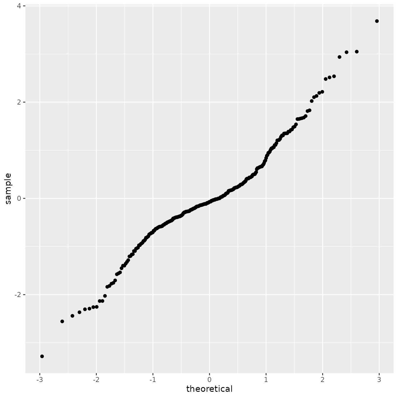
We will now do a parametric bootstrap procedure to obtain confidence bands (simulated envelopes) for the above QQ plot. We will consider \(B=100\) bootstrap samples. We start by generating \(B\) samples. This can be done by using the simulate() method:

B <- 100
samples_alpha2_bc <- simulate(fit_alpha2_bc, nsim = B)

To reduce computational cost, we will fix the latent parameters at the original fitted values, this can be done by passing the fitted model as the previous_fit argument, and setting fix_coeff to TRUE. We will compute the new standardized residuals based on these new samples:

simul_std_resid <- matrix(nrow = nrow(fitted_aug), ncol = B)
# We clone the graph to add new data
pems_graph_new <- pems_graph$clone()
for(i in 1:B){
  # We get the simulated response. Since we do not have replicates, 
  # all of them are in the first element of the list.
  y_tmp <- samples_alpha2_bc$samples[[1]][,i]
  # Add new observations
  pems_graph_new$add_observations(data = pems_graph$mutate(y = y_tmp), 
                                  clear_obs = TRUE, verbose = 0)
  new_fit <- graph_lme(y ~ 1, graph=pems_graph_new, BC = 1, 
                                previous_fit = fit_alpha2_bc,
                                model = list(type = "WhittleMatern", alpha = 2),
                                fix_coeff = TRUE)
  new_fitted_aug <-  augment(new_fit, se_fit = TRUE)        
  simul_std_resid[,i] <- new_fitted_aug[[".std_resid"]]            
}

We will now create the lower and upper bands with 95% confidence, as well as plot a median line. We being by extracting the lower, upper and median values.

  prob <- 0.95
  simul_std_resid <- t(simul_std_resid)
  simul_std_resid <- t(apply(simul_std_resid, 1, sort))
  simul_std_resid <- apply(simul_std_resid, 2, sort)
  id1 <- max(1, round(B * (1 - prob) / 2))
  id2 <- round(B * (1 + prob) / 2)
  bands <- rbind(simul_std_resid[id2, ], apply(simul_std_resid, 2, stats::median), simul_std_resid[id1, ])
  bands <- as.data.frame(t(bands))
  colnames(bands) <- c("upper", "median", "lower")  

Let us now produce the QQ plot with the confidence bands and median line. We start by obtaining the quantile values, and add them to the bands data.frame:

tmp_quantiles <- qqnorm(fitted_aug[[".std_resid"]])
bands[["x"]] <- sort(tmp_quantiles$x)
bands[["y"]] <- sort(tmp_quantiles$y)

p <- bands %>% ggplot(aes(x = x, y = y)) + geom_point() +
        geom_ribbon(aes(x = x, ymin = lower, ymax = upper), alpha = 0.2) +
        geom_path(aes(x=x, y = median), linetype = 2) + 
        labs(x = "Theoretical Quantiles", y = "Sample Quantiles")
p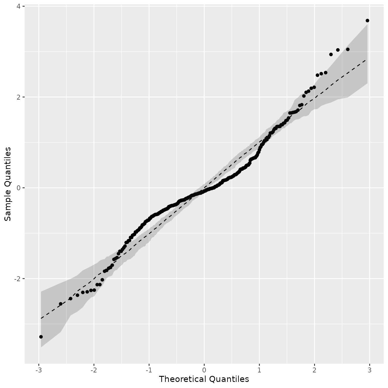

By observing the QQ plot with confidence bands, we can see that the Gaussianity assumption is reasonable; however, the fit can likely be improved by considering non-stationary Gaussian models as latent fields. However, it is not the goal of this vignette, as we are only comparing exact models. Our package has an implementation for nonstationary Gaussian models using finite element approximations.

References

Anderes, Ethan, Jesper Møller, and Jakob G Rasmussen. 2020. “Isotropic Covariance Functions on Graphs and Their Edges.” Annals of Statistics.

Bolin, David, Alexandre B. Simas, and Jonas Wallin. 2023. “Statistical Properties of Gaussian Whittle–Matérn Fields on Metric Graphs.” arXiv:2304.10372.

———. 2024. “Gaussian Whittle–Matérn Fields on Metric Graphs.” Bernoulli.

Borovitskiy, Viacheslav, Iskander Azangulov, Alexander Terenin, Peter Mostowsky, Marc Deisenroth, and Nicolas Durrande. 2021. “Matérn Gaussian Processes on Graphs.” International Conference on Artificial Intelligence and Statistics.