inlabru interface of Whittle--Matérn fields

Introduction

In this vignette we will present our inlabru interface to Whittle–Matérn fields. The underlying theory for this approach is provided in Bolin, Simas, and Wallin (2024) and Bolin, Simas, and Wallin (2023).

For an introduction to the metric_graph class, please see the Working with metric graphs vignette.

For handling data manipulation on metric graphs, see Data manipulation on metric graphs

For our R-INLA interface, see the INLA interface of Whittle–Matérn fields vignette.

In the Gaussian random fields on metric graphs vignette, we introduce all the models in metric graphs contained in this package, as well as, how to perform statistical tasks on these models, but without the R-INLA or inlabru interfaces.

We will present our inlabru interface to the Whittle-Matérn fields by providing a step-by-step illustration.

The Whittle–Matérn fields are specified as solutions to the stochastic differential equation $(\kappa^2 - \Delta)^{\alpha} \tau u = \mathcal{W}$ on the metric graph $\Gamma$ . We can work with these models without any approximations if the smoothness parameter $\alpha$ is an integer, and this is what we focus on in this vignette. For details on the case of a general smoothness parameter, see Whittle–Matérn fields with general smoothness.

A toy dataset

Let us begin by loading the MetricGraph package and creating a metric graph:

library(MetricGraph)

edge1 <- rbind(c(0,0),c(1,0))
edge2 <- rbind(c(0,0),c(0,1))
edge3 <- rbind(c(0,1),c(-1,1))
theta <- seq(from=pi,to=3*pi/2,length.out = 20)
edge4 <- cbind(sin(theta),1+ cos(theta))
edges = list(edge1, edge2, edge3, edge4)
graph_bru <- metric_graph$new(edges = edges)

Let us add 50 random locations in each edge where we will have observations:

obs_per_edge <- 50
obs_loc <- NULL
for(i in 1:(graph_bru$nE)) {
  obs_loc <- rbind(obs_loc,
                   cbind(rep(i,obs_per_edge), 
                   runif(obs_per_edge)))
}

We will now sample in these observation locations and plot the latent field:

sigma <- 2
alpha <- 1
nu <- alpha - 0.5
r <- 0.15 # r stands for range

u <- sample_spde(range = r, sigma = sigma, alpha = alpha,
                 graph = graph_bru, PtE = obs_loc)
graph_bru$plot(X = u, X_loc = obs_loc)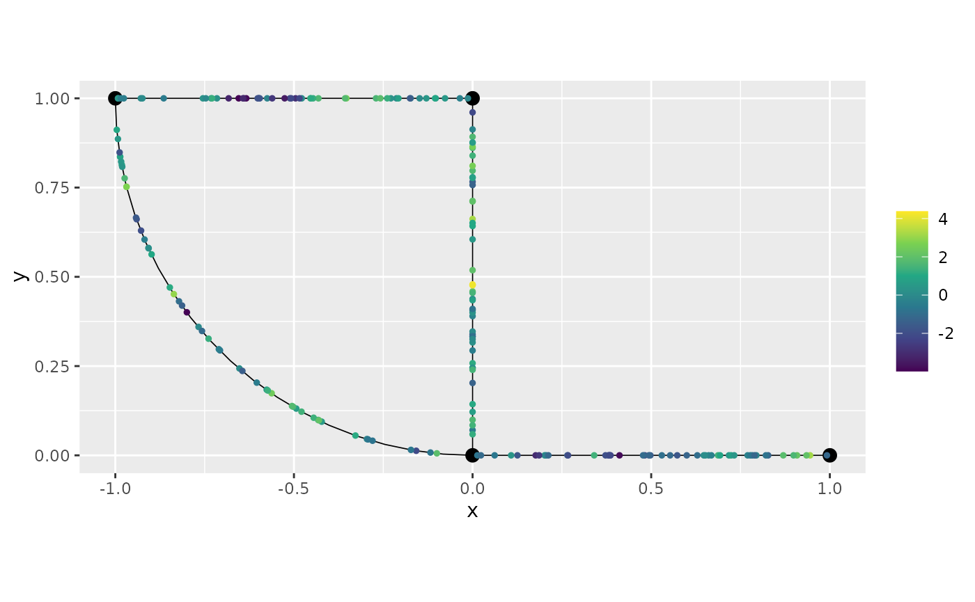

Let us now generate the observed responses, which we will call y. We will also plot the observed responses on the metric graph.

n_obs <- length(u)
sigma.e <- 0.1

y <- u + sigma.e * rnorm(n_obs)
graph_bru$plot(X = y, X_loc = obs_loc)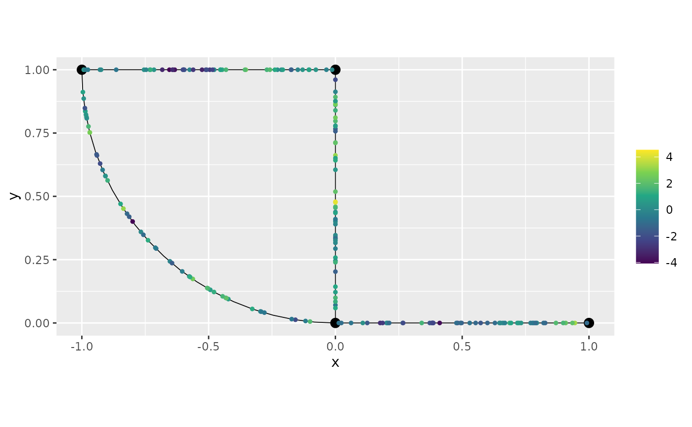

`inlabru` implementation

We will now present our inlabru implementation of the Whittle-Matérn fields for metric graphs. It has the advantage, over our R-INLA implementation, of not requiring the user to provide observation matrices, indices nor stack objects.

We are now in a position to fit the model with our inlabru implementation. Because of this, we need to add the observations to the graph, which we will do with the add_observations() method.

# Creating the data frame
df_graph <- data.frame(y = y, edge_number = obs_loc[,1],
                      distance_on_edge = obs_loc[,2])
# Adding observations and turning them to vertices
graph_bru$add_observations(data = df_graph, normalized=TRUE)

## Adding observations...

## list()

graph_bru$plot(data="y")

Now, we load INLA and inlabru packages. We will also need to create the inla model object with the graph_spde function. By default we have alpha=1.

library(INLA)
library(inlabru)
spde_model_bru <- graph_spde(graph_bru)

Now, we create inlabru’s component, which is a formula-like object. The index parameter in inlabru is not used in our implementation, thus, we replace it by the repl argument, which tells which replicates to use. If there is no replicates, we supply NULL.

cmp <-
    y ~ -1 + Intercept(1) + field(loc,
                    model = spde_model_bru)

Now, we create the data object to be passed to the bru() function:

data_spde_bru <- graph_data_spde(spde_model_bru, loc_name = "loc")

we directly fit the model by providing the data component of the data_spde_bru list:

spde_bru_fit <-
    bru(cmp, data=data_spde_bru[["data"]],
        options = list(num.threads = "1:1")
        )

Let us now obtain the estimates in the original scale by using the spde_metric_graph_result() function, then taking a summary():

spde_bru_result <- spde_metric_graph_result(spde_bru_fit, 
                    "field", spde_model_bru)

summary(spde_bru_result)

##            mean        sd 0.025quant  0.5quant 0.975quant      mode
## sigma 1.6497400 0.1351730  1.4027100 1.6437600    1.93306 1.6111200
## range 0.0864231 0.0170456  0.0584394 0.0844947    0.12515 0.0806159

We will now compare the means of the estimated values with the true values:

  result_df_bru <- data.frame(
    parameter = c("std.dev", "range"),
    true = c(sigma, r),
    mean = c(
      spde_bru_result$summary.sigma$mean,
      spde_bru_result$summary.range$mean
    ),
    mode = c(
      spde_bru_result$summary.sigma$mode,
      spde_bru_result$summary.range$mode
    )
  )
  print(result_df_bru)

##   parameter true       mean       mode
## 1   std.dev 2.00 1.64973907 1.61112427
## 2     range 0.15 0.08642314 0.08061591

We can also plot the posterior marginal densities with the help of the gg_df() function:

  posterior_df_bru_fit <- gg_df(spde_bru_result)

  library(ggplot2)

  ggplot(posterior_df_bru_fit) + geom_line(aes(x = x, y = y)) + 
  facet_wrap(~parameter, scales = "free") + labs(y = "Density")

Kriging with the `inlabru` implementation

Unfortunately, our inlabru implementation is not compatible with inlabru’s predict() method. This has to do with the nature of the metric graph’s object.

To this end, we have provided a different predict() method. We will now show how to do kriging with the help of this function.

We begin by creating a data list with the positions we want the predictions. In this case, we will want the predictions on a mesh.

Let us begin by obtaining an evenly spaced mesh with respect to the base graph:

obs_per_edge_prd <- 30
graph_bru$build_mesh(n = obs_per_edge_prd)

Let us plot the resulting graph:

graph_bru$plot(mesh=TRUE)

The positions we want are the mesh positions, which can be obtained by using the get_mesh_locations() method. We also set bru=TRUE and loc="loc" to obtain a data list suitable to be used with inlabru.

data_list <- graph_bru$get_mesh_locations(bru = TRUE,
                                            loc_name = "loc")

We can now obtain the predictions by using the predict() method. Observe that our predict() method for graph models is a bit different from inlabru’s standard predict() method. Indeed, the first argument is the model created with the graph_spde() function, the second is inlabru’s component, and the remaining is as done with the standard predict() method in inlabru.

field_pred <- predict(spde_model_bru, 
                                cmp,
                                spde_bru_fit, 
                                newdata = data_list,
                                formula = ~field)

## Warning in (function (formula = . ~ ., family = "gaussian", data = NULL, : Non data-frame list-like data supplied; guessing allow_combine=TRUE.
##   Specify allow_combine explicitly to avoid this warning.

Finally, we can plot the predictions together with the data:

plot(field_pred)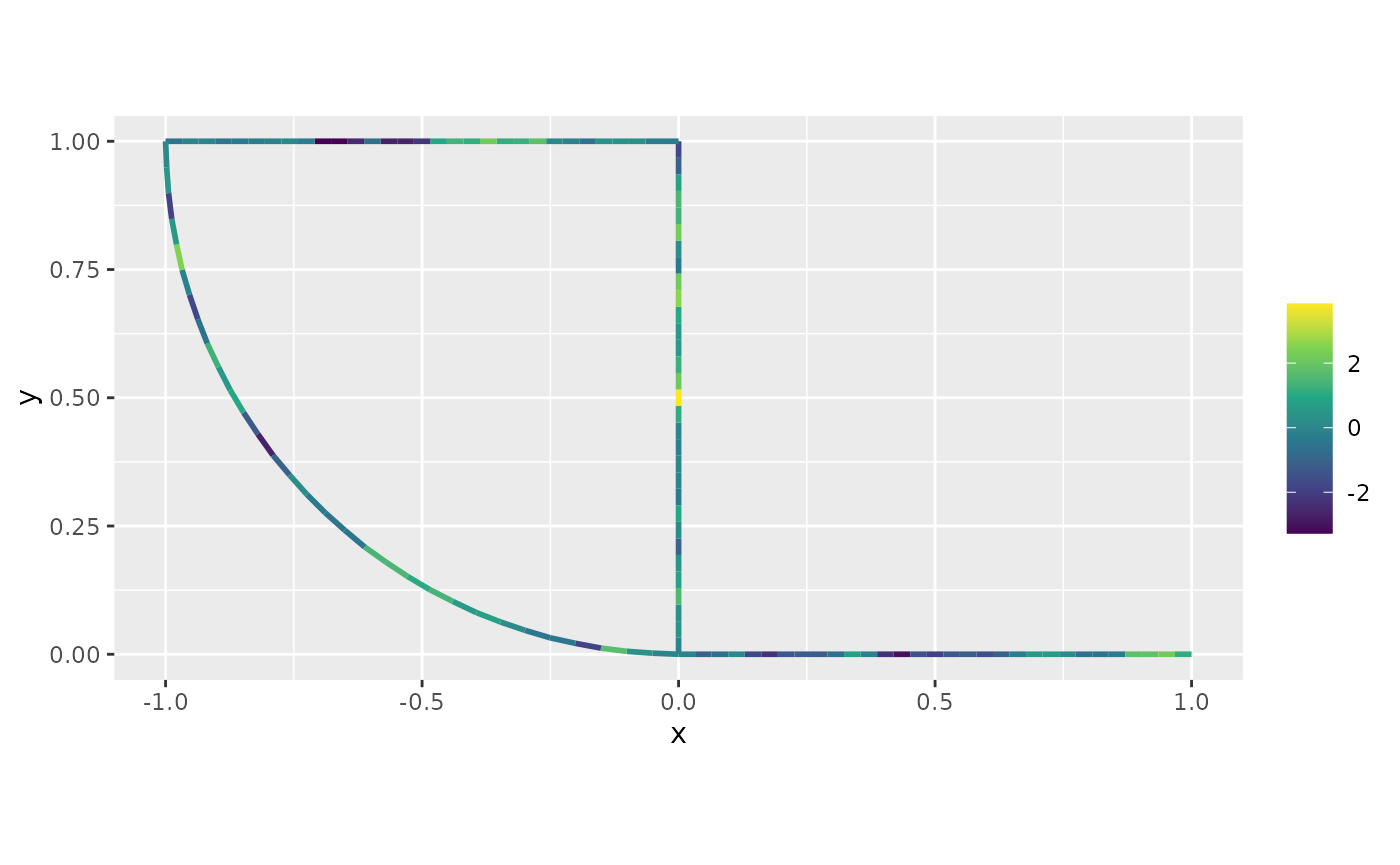

We can also obtain a 3d plot by setting plotly to TRUE:

plot(field_pred, type = "plotly")

An example with `alpha = 2`

We will now show an example where the parameter alpha is equal to 2. There is essentially no change in the commands above. Let us first clear the observations:

graph_bru$clear_observations()

Let us now simulate the data with alpha=2. We will now sample in these observation locations and plot the latent field:

sigma <- 2
alpha <- 2
nu <- alpha - 0.5
r <- 0.15 # r stands for range


u <- sample_spde(range = r, sigma = sigma, alpha = alpha,
                 graph = graph_bru, PtE = obs_loc)
graph_bru$plot(X = u, X_loc = obs_loc)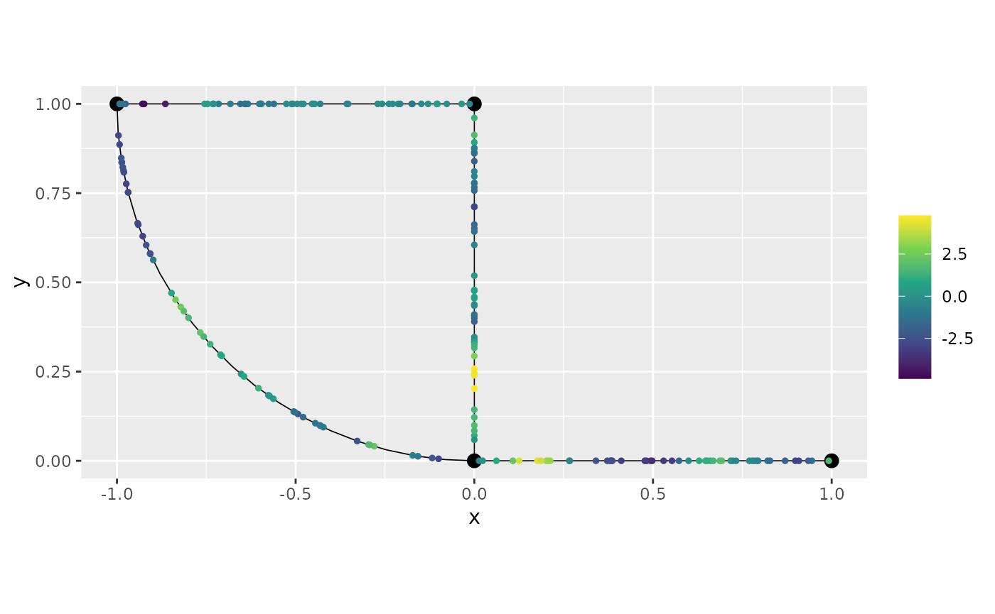

In the same way as before we will generate y and add the observations:

n_obs <- length(u)
sigma.e <- 0.1

y <- u + sigma.e * rnorm(n_obs)

df_graph <- data.frame(y = y, edge_number = obs_loc[,1],
                        distance_on_edge = obs_loc[,2])

graph_bru$add_observations(data=df_graph, normalized=TRUE)

## list()

Let us now create the model object for alpha=2:

spde_model_alpha2 <- graph_spde(graph_bru, alpha = 2)

Now, we will create the new data object with the graph_data_spde() function, in which we need to pass the argument loc_name that is needed for bru():

data_spde_alpha2 <- graph_data_spde(graph_spde = spde_model_alpha2, 
                            loc_name = "loc")

Now, we create inlabru’s component:

cmp_alpha2 <-
    y ~ -1 + Intercept(1) + field(loc,
                    model = spde_model_alpha2)

we directly fit the model by providing the data component of the data_spde_bru list:

spde_bru_fit_alpha2 <-
    bru(cmp_alpha2, data=data_spde_alpha2[["data"]],
    options = list(num.threads = "1:1"))

Let us now obtain the estimates in the original scale by using the spde_metric_graph_result() function, then taking a summary():

spde_bru_result_alpha2 <- spde_metric_graph_result(spde_bru_fit_alpha2, 
                    "field", spde_model_alpha2)

summary(spde_bru_result_alpha2)

##           mean        sd 0.025quant 0.5quant 0.975quant     mode
## sigma 2.023380 0.2287480   1.615870 2.010410   2.511980 1.976750
## range 0.152909 0.0169947   0.122271 0.151994   0.188938 0.150063

We will now compare the means of the estimated values with the true values:

  result_df_bru <- data.frame(
    parameter = c("std.dev", "range"),
    true = c(sigma, r),
    mean = c(
      spde_bru_result_alpha2$summary.sigma$mean,
      spde_bru_result_alpha2$summary.range$mean
    ),
    mode = c(
      spde_bru_result_alpha2$summary.sigma$mode,
      spde_bru_result_alpha2$summary.range$mode
    )
  )
  print(result_df_bru)

##   parameter true      mean      mode
## 1   std.dev 2.00 2.0233785 1.9767458
## 2     range 0.15 0.1529087 0.1500628

We can also plot the posterior marginal densities with the help of the gg_df() function:

  posterior_df_bru_fit <- gg_df(spde_bru_result_alpha2)

  library(ggplot2)

  ggplot(posterior_df_bru_fit) + geom_line(aes(x = x, y = y)) + 
  facet_wrap(~parameter, scales = "free") + labs(y = "Density")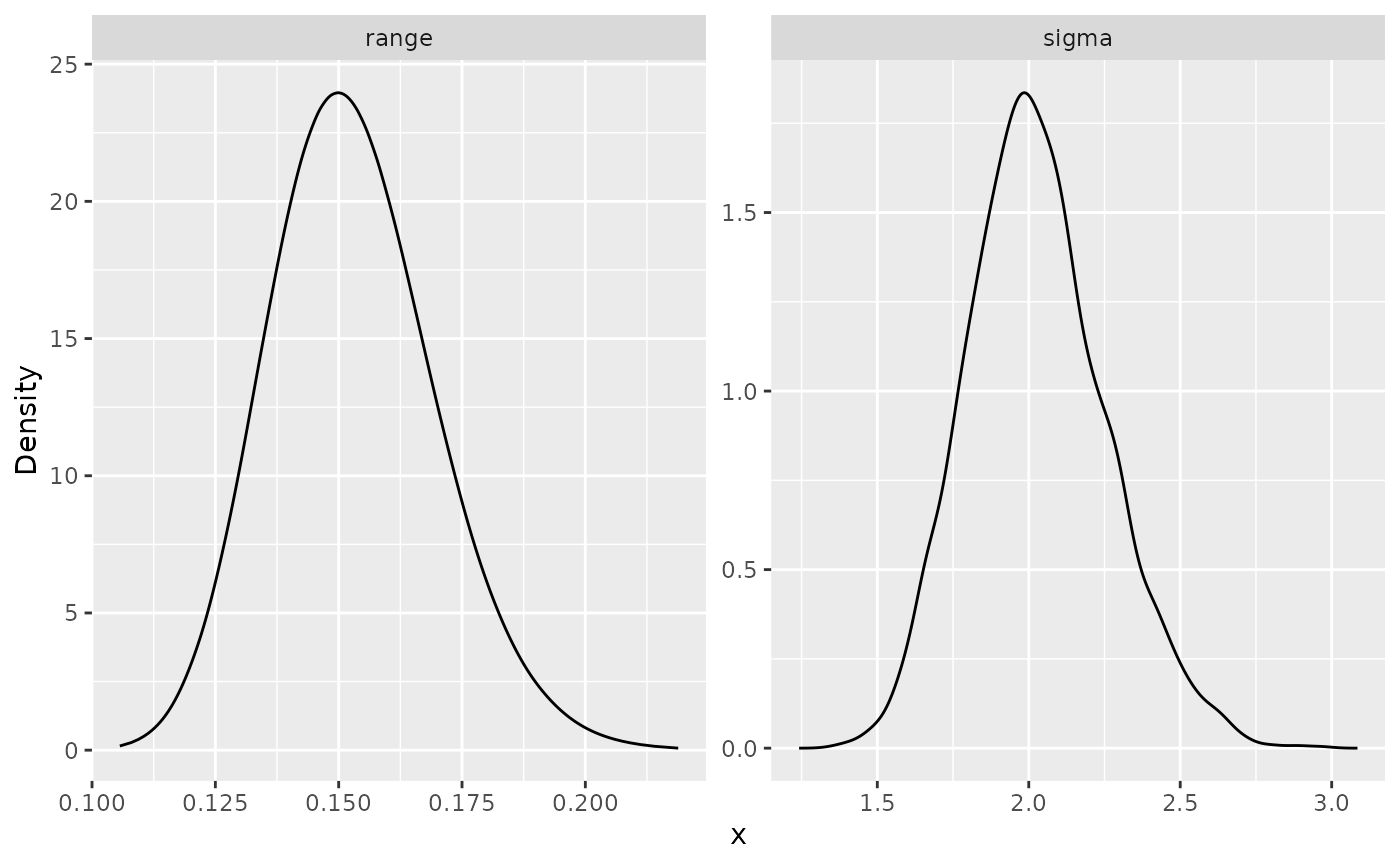

Let us now do prediction with alpha=2. We proceed as before, and we will use the same data list data_list to do prediction on the mesh locations. Thus, we will obtain predictions by using the predict() method. Observe that, again, we will use our predict method, instead of the default one from inlabru.

field_pred_alpha2 <- predict(spde_model_alpha2, 
                                cmp_alpha2,
                                spde_bru_fit_alpha2, 
                                newdata = data_list,
                                formula = ~field)

## Warning in (function (formula = . ~ ., family = "gaussian", data = NULL, : Non data-frame list-like data supplied; guessing allow_combine=TRUE.
##   Specify allow_combine explicitly to avoid this warning.

Finally, we can plot the predictions together with the data:

plot(field_pred_alpha2)

We can also obtain a 3d plot by setting plotly to TRUE:

plot(field_pred_alpha2, type = "plotly")

Fitting `inlabru` models with replicates

We will now illustrate how to use our inlabru implementation to fit models with replicates.

To simplify exposition, we will use the same base graph. So, we begin by clearing the observations:

graph_bru$clear_observations()

We will use the same observation locations as for the previous cases. Let us sample 30 replicates:

sigma_rep <- 1.5
alpha_rep <- 1
nu_rep <- alpha_rep - 0.5
r_rep <- 0.2 # r stands for range

n_repl <- 30

u_rep <- sample_spde(range = r_rep, sigma = sigma_rep,
                 alpha = alpha_rep,
                 graph = graph_bru, PtE = obs_loc,
                 nsim = n_repl)

Let us now generate the observed responses, which we will call y_rep.

n_obs_rep <- nrow(u_rep)
sigma_e <- 0.1

y_rep <- u_rep + sigma_e * matrix(rnorm(n_obs_rep * n_repl),
                                    ncol=n_repl)

We can now add the the observations by setting the group argument to repl:

dl_rep_graph <- lapply(1:ncol(y_rep), function(i){data.frame(y = y_rep[,i],
                                          edge_number = obs_loc[,1],
                                          distance_on_edge = obs_loc[,2],
                                          repl = i)})
dl_rep_graph <- do.call(rbind, dl_rep_graph)

graph_bru$add_observations(data = dl_rep_graph, normalized=TRUE,
                                    group = "repl")

## Adding observations...

## list()

By definition the plot() method plots the first replicate. We can select the other replicates with the group argument. See the Working with metric graphs for more details.

graph_bru$plot(data="y")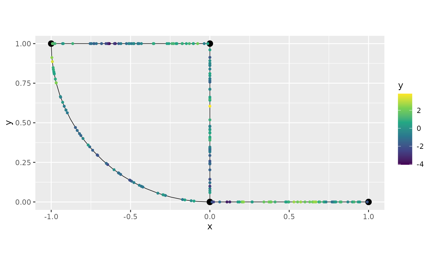

Let us plot another replicate:

graph_bru$plot(data="y", group=2)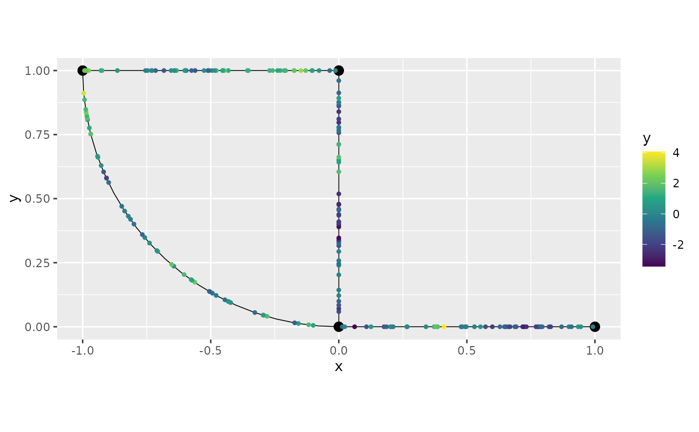

Let us now create the model object:

spde_model_bru_rep <- graph_spde(graph_bru)

Let us first create a model using the replicates 1, 3, 5, 7 and 9. To this end, we provide the vector of the replicates we want as the input argument to the field. The graph_data_spde() acts as a helper function when building this vector. All we need to do, is to use the repl component of the list created when using the graph_data_spde()

data_spde_bru <- graph_data_spde(spde_model_bru_rep, 
        loc_name = "loc",
        repl=c(1,3,5,7,9),
        repl_col = "repl")

repl <- data_spde_bru[["repl"]]
cmp_rep <-
    y ~ -1 + Intercept(1) + field(loc, 
                        model = spde_model_bru_rep,
                        replicate = repl)

Now, we fit the model:

spde_bru_fit_rep <-
    bru(cmp_rep,
        data=data_spde_bru[["data"]],
        options=list(
        num.threads = "1:1")
    )

## Warning in (function (formula = . ~ ., family = "gaussian", data = NULL, : Non data-frame list-like data supplied; guessing allow_combine=TRUE.
##   Specify allow_combine explicitly to avoid this warning.

Let us see the estimated values in the original scale:

spde_result_bru_rep <- spde_metric_graph_result(spde_bru_fit_rep, 
                        "field", spde_model_bru_rep)

summary(spde_result_bru_rep)

##           mean        sd 0.025quant 0.5quant 0.975quant     mode
## sigma 1.467660 0.0717155   1.334060 1.465610   1.614850 1.463360
## range 0.190249 0.0214184   0.152153 0.188815   0.236234 0.185799

Let us compare with the true values:

  result_df_bru_rep <- data.frame(
    parameter = c("std.dev", "range"),
    true = c(sigma_rep, r_rep),
    mean = c(
      spde_result_bru_rep$summary.sigma$mean,
      spde_result_bru_rep$summary.range$mean
    ),
    mode = c(
      spde_result_bru_rep$summary.sigma$mode,
      spde_result_bru_rep$summary.range$mode
    )
  )
  print(result_df_bru_rep)

##   parameter true      mean     mode
## 1   std.dev  1.5 1.4676557 1.463364
## 2     range  0.2 0.1902489 0.185799

We will now show how to fit the model considering all replicates. To this end, we simply set the repl argument in graph_data_spde() function to .all.

data_spde_bru_rep <- graph_data_spde(spde_model_bru_rep, 
        loc_name = "loc",
        repl=".all",
        repl_col = "repl")

repl <- data_spde_bru_rep[["repl"]]

cmp_rep <-  y ~ -1 + Intercept(1) + field(loc, 
                        model = spde_model_bru_rep,
                        replicate = repl)

Similarly, we fit the model, by setting the repl argument to “.all” inside the graph_data_spde() function:

spde_bru_fit_rep <-
    bru(cmp_rep,
        data=data_spde_bru_rep[["data"]],
        options=list(
        num.threads = "1:1")
    )

## Warning in (function (formula = . ~ ., family = "gaussian", data = NULL, : Non data-frame list-like data supplied; guessing allow_combine=TRUE.
##   Specify allow_combine explicitly to avoid this warning.

Let us see the estimated values in the original scale:

spde_result_bru_rep <- spde_metric_graph_result(spde_bru_fit_rep, 
                        "field", spde_model_bru_rep)

summary(spde_result_bru_rep)

##           mean         sd 0.025quant 0.5quant 0.975quant     mode
## sigma 1.488410 0.02963520   1.431450  1.48803   1.547530 1.487930
## range 0.191687 0.00865412   0.175417  0.19141   0.209439 0.190786

Let us compare with the true values:

  result_df_bru_rep <- data.frame(
    parameter = c("std.dev", "range"),
    true = c(sigma_rep, r_rep),
    mean = c(
      spde_result_bru_rep$summary.sigma$mean,
      spde_result_bru_rep$summary.range$mean
    ),
    mode = c(
      spde_result_bru_rep$summary.sigma$mode,
      spde_result_bru_rep$summary.range$mode
    )
  )
  print(result_df_bru_rep)

##   parameter true      mean     mode
## 1   std.dev  1.5 1.4884077 1.487930
## 2     range  0.2 0.1916873 0.190786

An application with real data

For this example we will consider the pems data contained in the MetricGraph package. This data was illustrated in (Bolin, Simas, and Wallin 2023). The data consists of traffic speed observations on highways in the city of San Jose, California. The traffic speeds are stored in the variable y. We will also add the observations to the metric graph object:

pems_graph <- metric_graph$new(edges=pems$edges)
pems_graph$add_observations(data=pems$data)

## list()

pems_graph$prune_vertices()

Let us now plot the data. We will choose the data such that longitude is between -121.905 and 121.875, and latitude is between 37.312 and 37.328:

p <- pems_graph$filter(-121.905< .coord_x, .coord_x < -121.875,
                          37.312 < .coord_y, .coord_y < 37.328) %>%
                          pems_graph$plot(data="y", vertex_size=0,
                                          data_size=4)
      p + xlim(-121.905,-121.875) + ylim(37.312,37.328)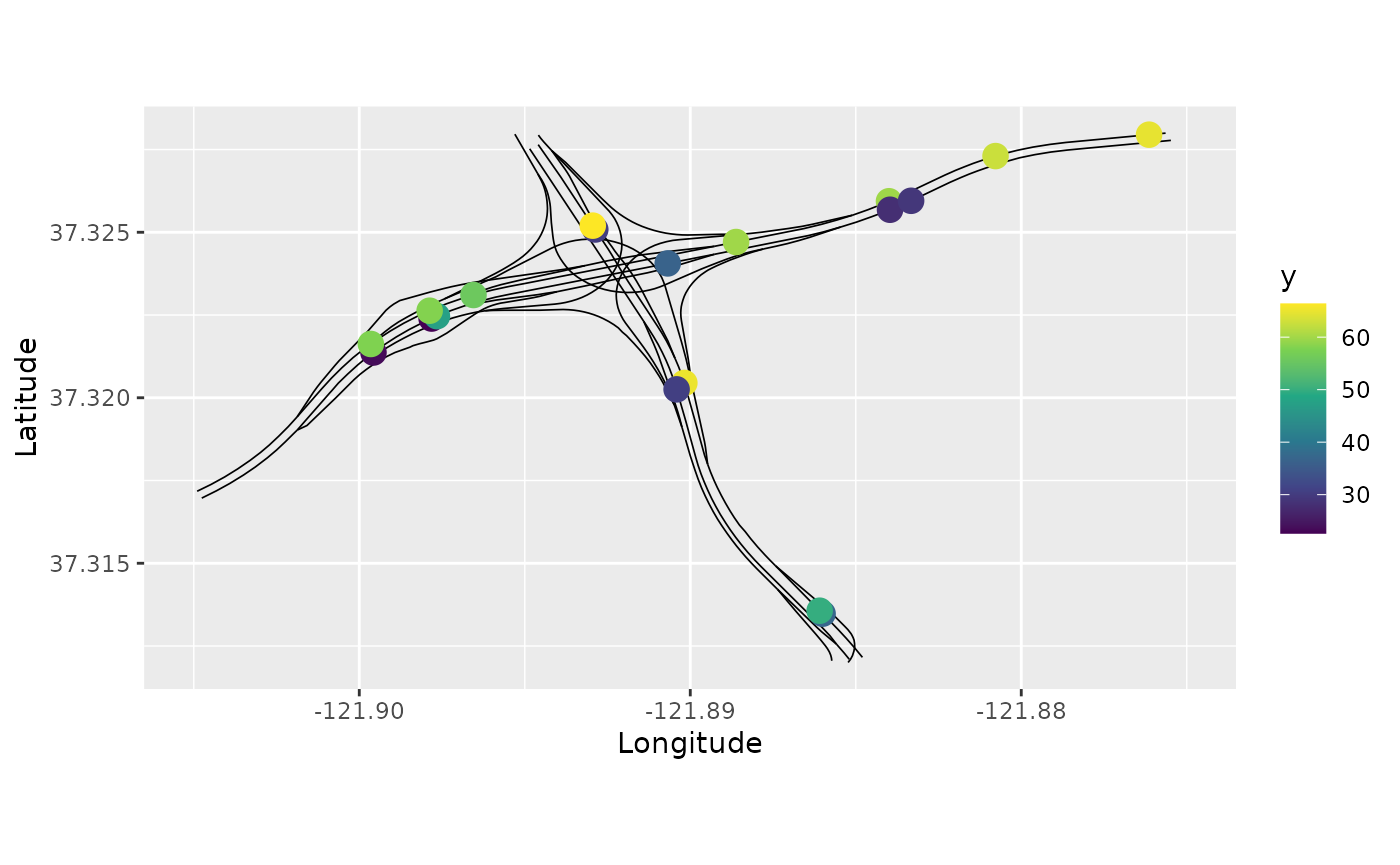

We will now create and fit models with both $\alpha=1$ and $\alpha=2$ using inlabru:

# Model with alpha = 1
spde_model_bru_pems_1 <- graph_spde(pems_graph, alpha=1)
cmp_1 <- y ~ -1 + Intercept(1) + field(loc, 
                                  model = spde_model_bru_pems_1)
data_spde_bru_pems_1 <- graph_data_spde(spde_model_bru_pems_1, loc_name = "loc")
spde_bru_fit_pems_1 <- bru(cmp_1, data=data_spde_bru_pems_1[["data"]], 
                          options=list(num.threads = "1:1"))

## Warning in (function (formula = . ~ ., family = "gaussian", data = NULL, : Non data-frame list-like data supplied; guessing allow_combine=TRUE.
##   Specify allow_combine explicitly to avoid this warning.

# Model with alpha = 2
spde_model_bru_pems_2 <- graph_spde(pems_graph, alpha=2, start_sigma = 10)
cmp_2 <- y ~ -1 + Intercept(1) + field(loc, 
                                    model = spde_model_bru_pems_2)
data_spde_bru_pems_2 <- graph_data_spde(spde_model_bru_pems_2, loc_name = "loc")
spde_bru_fit_pems_2 <- bru(cmp_2, data=data_spde_bru_pems_2[["data"]], 
                          options=list(num.threads = "1:1"))

## Warning in (function (formula = . ~ ., family = "gaussian", data = NULL, : Non data-frame list-like data supplied; guessing allow_combine=TRUE.
##   Specify allow_combine explicitly to avoid this warning.

Let us see the estimated values in the original scale for both models:

# Results for alpha = 1
spde_result_bru_pems_1 <- spde_metric_graph_result(spde_bru_fit_pems_1, 
                        "field", spde_model_bru_pems_1)
cat("Results for alpha = 1:\n")

## Results for alpha = 1:

summary(spde_result_bru_pems_1)

##           mean       sd 0.025quant 0.5quant 0.975quant    mode
## sigma  45.8087  30.3644    17.6012  37.0613    128.316 27.0966
## range 142.5190 280.8360    15.7554  61.3415    792.135 24.7037

# Results for alpha = 2
spde_result_bru_pems_2 <- spde_metric_graph_result(spde_bru_fit_pems_2, 
                        "field", spde_model_bru_pems_2)
cat("\nResults for alpha = 2:\n")

## 
## Results for alpha = 2:

summary(spde_result_bru_pems_2)

##           mean      sd 0.025quant 0.5quant 0.975quant     mode
## sigma 21.02920 3.27505   15.42050 20.77290    28.2349 19.94330
## range  8.85058 1.57738    6.13893  8.72013    12.3173  8.46142

We can now get the mesh locations to do prediction. We start by creating a mesh and extracting the indexes of the mesh such that longitude is between -121.905 and 121.875, and latitude is between 37.312 and 37.328:

pems_graph$build_mesh(h=0.1)

# Getting mesh coordinates
mesh_coords <- pems_graph$mesh$V

# Finding coordinates such that longitude is between 
# `-121.905` and `121.875`, and latitude is between `37.312` and `37.328`
idx_x <- (mesh_coords[,1] > -121.905) & (mesh_coords[,1] < -121.875)
idx_y <- (mesh_coords[,2] > 37.312) & (mesh_coords[,2] < 37.328)
idx_xy <- idx_x & idx_y

# Create prediction data list
pred_coords <- list()
pred_coords[["loc"]] <- pems_graph$mesh$VtE[idx_xy,]

Finally, we will do prediction and plot them for the model with alpha=1.

field_pred_pems_1 <- predict(spde_model_bru_pems_1, cmp_1, 
                        spde_bru_fit_pems_1,
                        newdata = pred_coords,
                        formula = ~ Intercept + field)

cat("Predictions for alpha = 1:\n")

## Predictions for alpha = 1:

plot(field_pred_pems_1, edge_width = 0.5, vertex_size = 0) +
      xlim(-121.905,-121.875) + ylim(37.316,37.328)

Bolin, David, Alexandre B. Simas, and Jonas Wallin. 2023. “Statistical Properties of Gaussian Whittle–Matérn Fields on Metric Graphs.” arXiv:2304.10372.

———. 2024. “Gaussian Whittle–Matérn Fields on Metric Graphs.” Bernoulli 30: 1611–39.

David Bolin, Alexandre B. Simas, and Jonas Wallin

Created: 2022-11-23. Last modified: 2024-12-13.

Introduction

A toy dataset

`inlabru` implementation

Kriging with the `inlabru` implementation

An example with `alpha = 2`

Fitting `inlabru` models with replicates

An application with real data

inlabru interface of Whittle--Matérn fields

David Bolin, Alexandre B. Simas, and Jonas Wallin

Created: 2022-11-23. Last modified: 2024-12-13.

Introduction

A toy dataset

inlabru implementation

Kriging with the inlabru implementation

An example with alpha = 2

Fitting inlabru models with replicates

An application with real data

`inlabru` implementation

Kriging with the `inlabru` implementation

An example with `alpha = 2`

Fitting `inlabru` models with replicates