Log-Gaussian Cox processes on metric graphs
David Bolin, Alexandre B. Simas, and Jonas Wallin
Created: 2023-01-30. Last modified: 2026-05-14.
Source:vignettes/pointprocess.Rmd
pointprocess.RmdIntroduction
In this vignette we will introduce how to work with log-Gaussian Cox
processes based on Whittle–Matérn fields on metric graphs. To simplify
the integration with R-INLA and inlabru hese
models are constructed using finite element approximations as
implemented in the rSPDE package. The theoretical details
will be given in the forthcoming article (Bolin
et al. 2023).
Constructing the graph and the mesh
We begin by loading the rSPDE, MetricGraph
and INLA packages:
library(rSPDE)
library(MetricGraph)
library(INLA)
As an example, we consider the default graph in the package:
graph <- metric_graph$new(tolerance = list(vertex_vertex = 1e-1, vertex_edge = 1e-3, edge_edge = 1e-3),
                          remove_deg2 = TRUE)
graph$plot()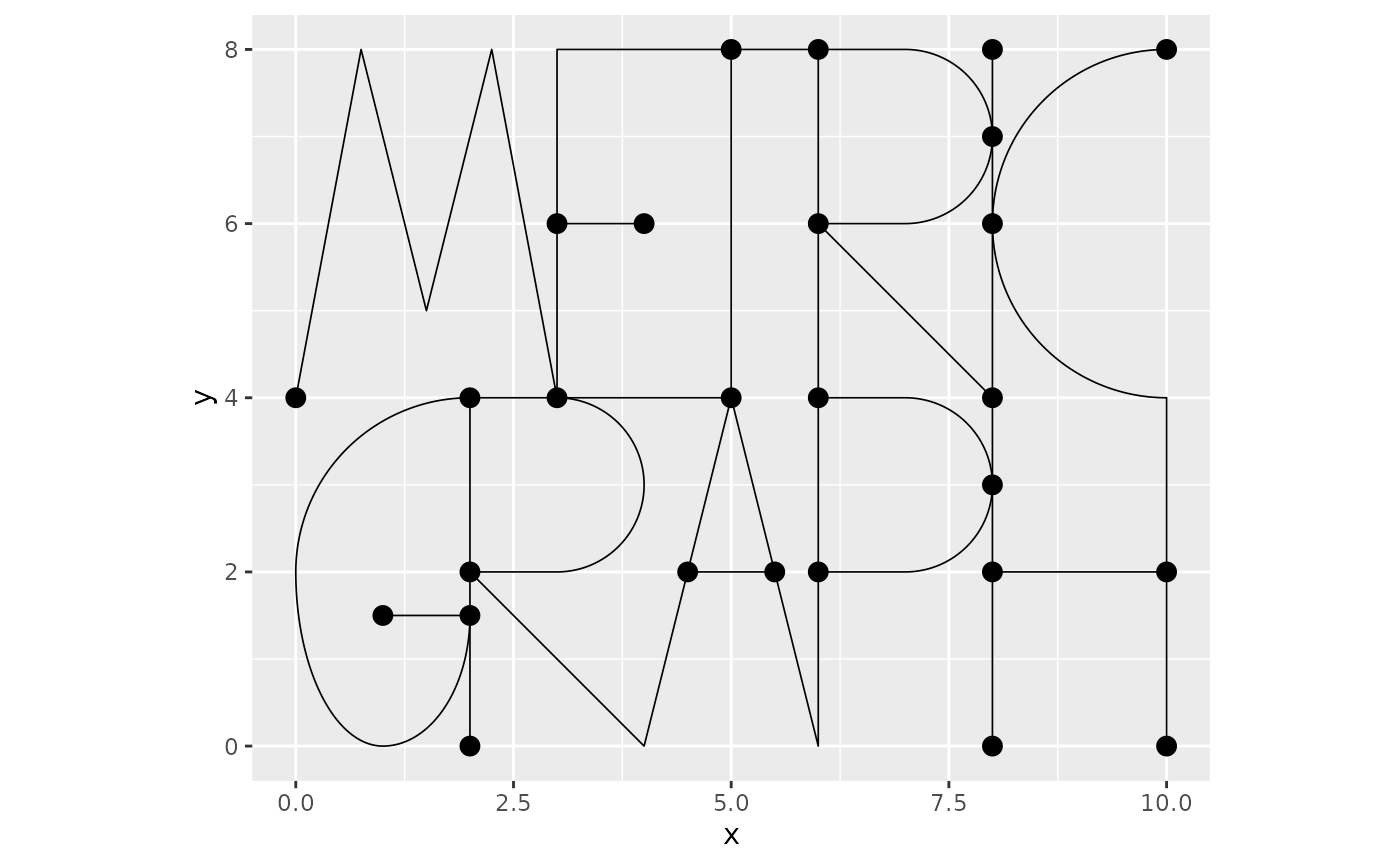
To construct a FEM approximation of a Whittle–Matérn field, we must first construct a mesh on the graph.
graph$build_mesh(h = 0.1)
graph$plot(mesh=TRUE)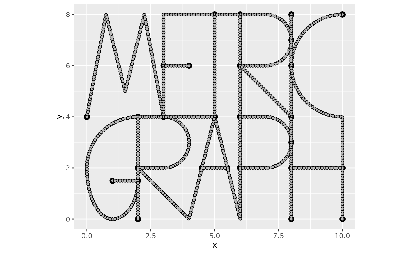
The next step is to build the mass and stiffness matrices for the FEM basis.
graph$compute_fem()We are now ready to specify the and sample from a log-Gaussian Cox
process model with intensity
where
is an intercept and
is a Gaussian Whittle–Matérn field specified by
For this we can use the function
graph_lgcp as follows:
  sigma <- 0.5
  range <- 2
  alpha <- 2
  cov_lgcp <- graph$mesh$VtE[,1]/max(graph$mesh$VtE[,1])
  lgcp_sample <- graph_lgcp_sim(intercept = -1 + 2*cov_lgcp, sigma = sigma,
                            range = range, alpha = alpha,
                            graph = graph)
The object returned by the function is a list with the simulated Gaussian process and the points on the graph. We can plot the simulated intensity function as
graph$plot_function(X = exp(lgcp_sample$u), vertex_size = 0)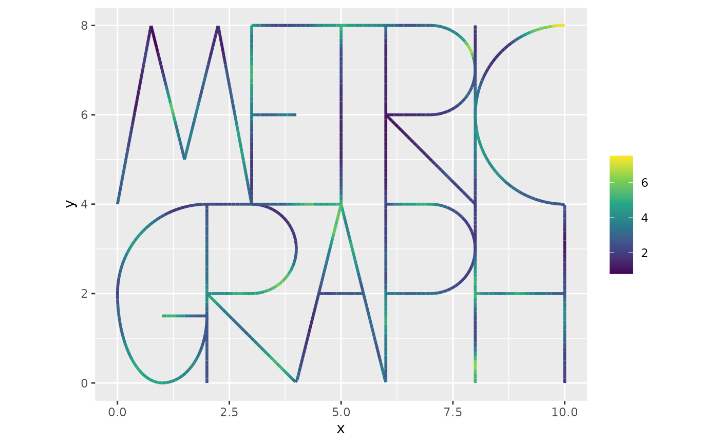
To plot the simulated points, we can add them to the graph and then plot:
graph$add_observations(data = data.frame(y=rep(1,length(lgcp_sample$edge_loc)),
                                         edge_number = lgcp_sample$edge_number,
                                         distance_on_edge = lgcp_sample$edge_loc,
                                         cov_lgcp = lgcp_sample$edge_number),
                       normalized = TRUE)
## Adding observations...## Assuming the observations are normalized by the length of the edge.
graph$plot(vertex_size = 0, data = "y")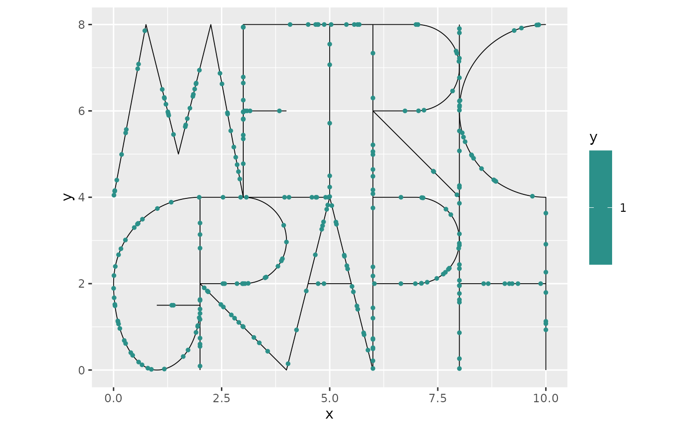
In order to fit a log-Gaussian Cox process model, we need to specify
integration points on the graph, be able to evaluate the covariates at
such integration points. This process is a bit involved, so we have
created an interface to simplify the process. In this interface, by
default, the covariates are interpolated from the data provided in the
graph object to obtain their values at the integration
points.
The integration points are defined, by default, as the mesh locations if the metric graph object has a mesh. If the mesh is not provided, one must either provide the integration points manually or build a mesh.
At the end of the vignette, we will also show how to fit the model in
INLA without using our INLA interface for LGCP
models.
Fitting LGCP models with our INLA interface
We will now fit the model using our INLA interface. To
such an end, we will clear the observations from the graph and add the
data to the graph.
graph$clear_observations()

#Add the data together with the exposure terms
graph$add_observations(data = data.frame(y = rep(1,length(lgcp_sample$edge_loc)),
                                         edge_number = lgcp_sample$edge_number,
                                         distance_on_edge = lgcp_sample$edge_loc,
                                         Intercept = 1,
                                         cov_lgcp = lgcp_sample$edge_number/max(lgcp_sample$edge_number)),
                       normalized = TRUE)
## Adding observations...## Assuming the observations are normalized by the length of the edge.We have added the response variable , however, this is not strictly necessary. If such a response variable is not provided, it will be assumed that all locations correspond to observed points.
Let us now create the rSPDE model object:
rspde_model <- rspde.metric_graph(graph, nu = alpha - 1/2)We can now fit the model using the lgcp_graph()
function:
inla_fit <- lgcp_graph(y ~ -1 + Intercept + cov_lgcp +
                      f(field, model = rspde_model), graph=graph)
Let us observe the inla_fit object:
summary(inla_fit)## Time used:
## Pre = 0.307, Running = 0.54, Post = 0.0509, Total = 0.898
## Fixed effects:
## mean sd 0.025quant 0.5quant 0.975quant mode kld
## Intercept -0.549 0.315 -1.183 -0.545 0.058 -0.545 0
## cov_lgcp 1.043 0.475 0.112 1.042 1.980 1.042 0
##
## Random effects:
## Name Model
## field CGeneric
##
## Model hyperparameters:
## mean sd 0.025quant 0.5quant 0.975quant mode
## Theta1 for field -0.701 0.305 -1.345 -0.687 -0.15 -0.616
## Theta2 for field 0.800 0.635 -0.498 0.817 2.00 0.890
##
## Marginal log-Likelihood: -106.72
## is computed
## Posterior summaries for the linear predictor and the fitted values are computed
## (Posterior marginals needs also 'control.compute=list(return.marginals.predictor=TRUE)')Let us extract the estimates in the original scale by using the
spde_metric_graph_result() function, then taking a
summary():
spde_result <- spde_metric_graph_result(inla_fit, "field", rspde_model)

summary(spde_result)
## mean sd 0.025quant 0.5quant 0.975quant mode
## std.dev 0.518762 0.153425 0.262207 0.505776 0.857188 0.477153
## range 2.700780 1.770700 0.615952 2.273870 7.318800 1.517510We will now compare the means of the estimated values with the true values:
  result_df <- data.frame(
    parameter = c("std.dev", "range"),
    true = c(sigma, range),
    mean = c(
      spde_result$summary.std.dev$mean,
      spde_result$summary.range$mean
    ),
    mode = c(
      spde_result$summary.std.dev$mode,
      spde_result$summary.range$mode
    )
  )
  print(result_df)
## parameter true mean mode
## 1 std.dev 0.5 0.5187621 0.477153
## 2 range 2.0 2.7007788 1.517507If we have the actual values of the covariates at the integration
points, we can pass them to the lgcp_graph() function via
the manual_covariates argument.
manual_covariates <- data.frame(Intercept = 1,
                      cov_lgcp = graph$mesh$VtE[,1]/max(lgcp_sample$edge_number),
                      .group = 1)
inla_fit <- lgcp_graph(y ~ -1 + Intercept + cov_lgcp + f(field, model = rspde_model),
             graph=graph, manual_covariates = manual_covariates, interpolate = FALSE)
Let us observe the new inla_fit object:
summary(inla_fit)## Time used:
## Pre = 0.141, Running = 0.509, Post = 0.027, Total = 0.677
## Fixed effects:
## mean sd 0.025quant 0.5quant 0.975quant mode kld
## Intercept -0.903 0.291 -1.50 -0.896 -0.352 -0.896 0
## cov_lgcp 1.905 0.398 1.14 1.899 2.707 1.899 0
##
## Random effects:
## Name Model
## field CGeneric
##
## Model hyperparameters:
## mean sd 0.025quant 0.5quant 0.975quant mode
## Theta1 for field -0.951 0.410 -1.837 -0.925 -0.239 -0.792
## Theta2 for field 1.035 0.737 -0.472 1.054 2.430 1.137
##
## Marginal log-Likelihood: -97.83
## is computed
## Posterior summaries for the linear predictor and the fitted values are computed
## (Posterior marginals needs also 'control.compute=list(return.marginals.predictor=TRUE)')We can now extract the estimates in the original scale
spde_result <- spde_metric_graph_result(inla_fit, "field", rspde_model)

summary(spde_result)
## mean sd 0.025quant 0.5quant 0.975quant mode
## std.dev 0.418133 0.162334 0.160838 0.400456 0.784069 0.354264
## range 3.649210 2.841910 0.633685 2.884500 11.237300 1.643790We can also plot the posterior marginal densities with the help of
the gg_df() function:
  posterior_df_fit <- gg_df(spde_result)

  library(ggplot2)

  ggplot(posterior_df_fit) + geom_line(aes(x = x, y = y)) +
  facet_wrap(~parameter, scales = "free") + labs(y = "Density")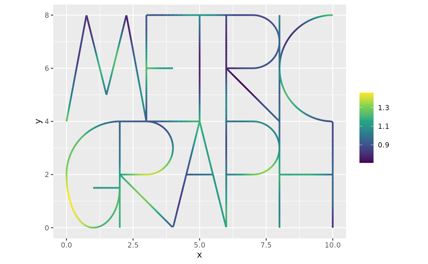
Finally, we can plot the estimated field :
n.obs <- length(graph$get_data()$y)
n.field <- dim(graph$mesh$VtE)[1]
u_posterior <- inla_fit$summary.linear.predictor$mean[(n.obs+1):(n.obs+n.field)]
graph$plot_function(X = u_posterior, vertex_size = 0)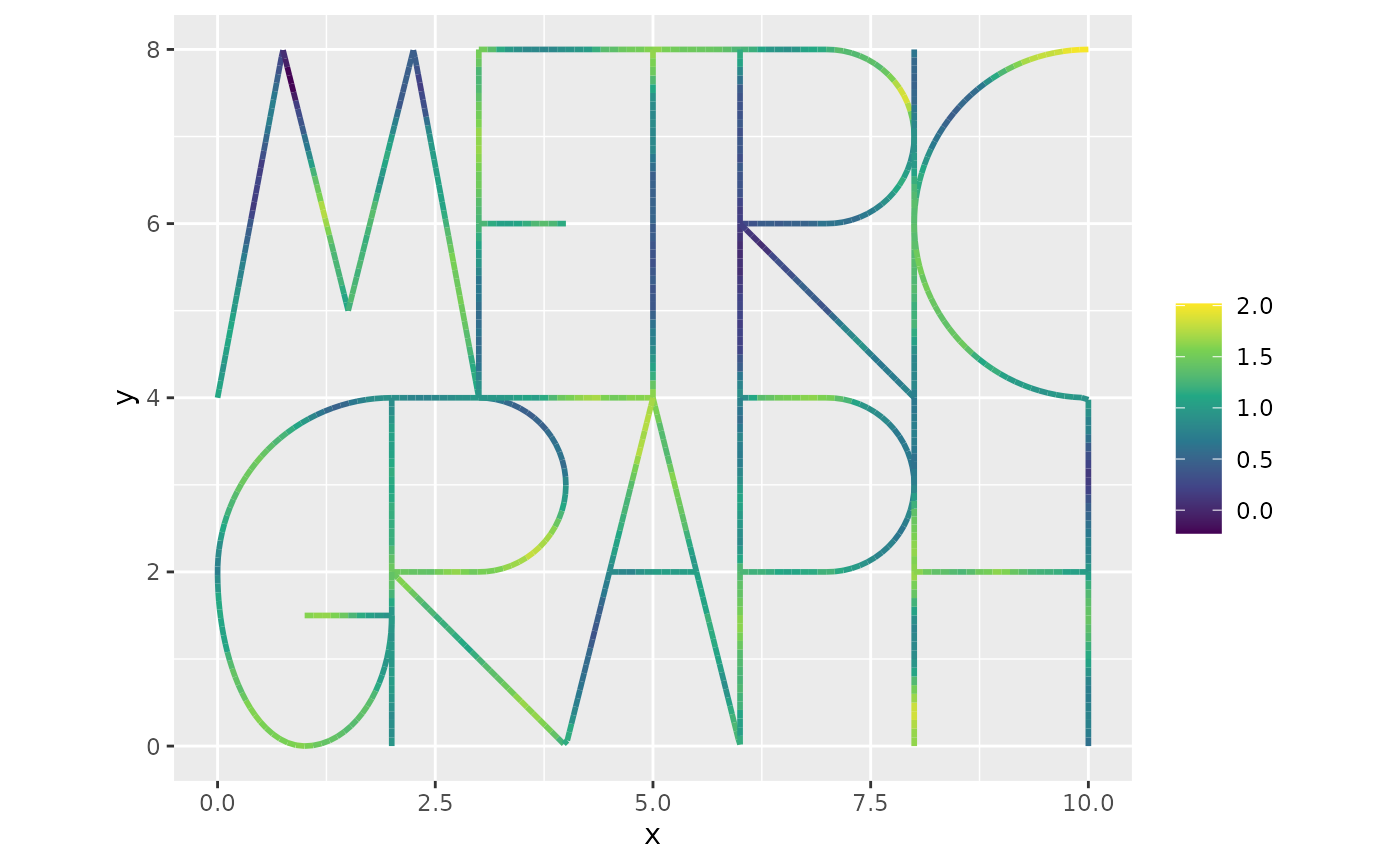
This can be compared with the field that was used to generate the data:
graph$plot_function(X = lgcp_sample$u, vertex_size = 0)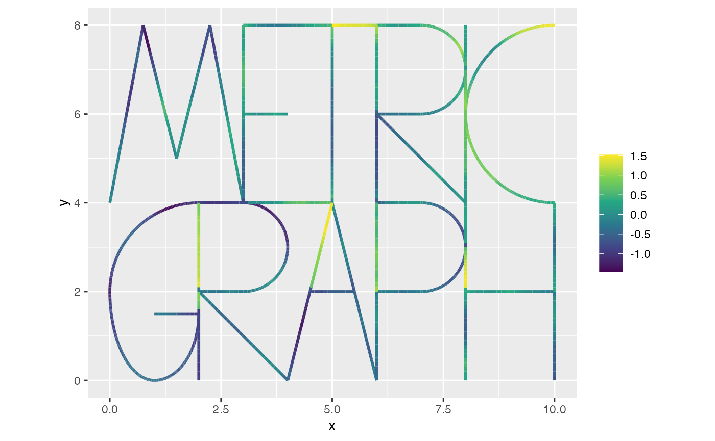
We can also fit the model using the exact model by using the
graph_spde() function as the SPDE model, and we also set
the LGCP argument to TRUE:
spde_model <- graph_spde(graph, alpha = 1, LGCP = TRUE)Let us now fit the model:
inla_fit_spde <- lgcp_graph(y ~ -1 + Intercept + cov_lgcp +
                          f(field, model = spde_model), graph=graph)
Let us observe the new inla_fit_spde object:
summary(inla_fit_spde)## Time used:
## Pre = 0.142, Running = 0.565, Post = 0.0294, Total = 0.736
## Fixed effects:
## mean sd 0.025quant 0.5quant 0.975quant mode kld
## Intercept -0.512 0.250 -1.002 -0.512 -0.023 -0.512 0
## cov_lgcp 1.050 0.403 0.261 1.050 1.839 1.050 0
##
## Random effects:
## Name Model
## field CGeneric
##
## Model hyperparameters:
## mean sd 0.025quant 0.5quant 0.975quant mode
## Theta1 for field 1.37 0.876 -0.276 1.34 3.170 1.23
## Theta2 for field -1.75 1.430 -4.706 -1.71 0.915 -1.50
##
## Marginal log-Likelihood: -105.40
## is computed
## Posterior summaries for the linear predictor and the fitted values are computed
## (Posterior marginals needs also 'control.compute=list(return.marginals.predictor=TRUE)')We can now extract the estimates in the original scale
spde_result <- spde_metric_graph_result(inla_fit_spde, "field", spde_model)

summary(spde_result)
## mean sd 0.025quant 0.5quant 0.975quant mode
## sigma 2.412320 0.734944 1.22946000 2.333300 4.09447 2.2614400
## range 0.433998 0.792698 0.00934058 0.183881 2.44873 0.0174288An example with replicates in our INLA interface
We start by simulating the data.
  n.rep <- 5
  sigma <- 0.5
  range <- 2
  alpha <- 2
  cov_lgcp <- graph$mesh$VtE[,1]/max(graph$mesh$VtE[,1])
  max_edge_num <- max(graph$mesh$VtE[,1])
  lgcp_sample_rep <- graph_lgcp_sim(n = n.rep, intercept = -1 + 2*cov_lgcp, sigma = sigma,
                            range = range, alpha = alpha,
                            graph = graph)
Let us clear the observations from the graph and add the simulated data.
graph$clear_observations()

df_rep <- data.frame(y=rep(1,length(lgcp_sample_rep[[1]]$edge_loc)),
                     edge_number = lgcp_sample_rep[[1]]$edge_number,
                     distance_on_edge = lgcp_sample_rep[[1]]$edge_loc,
                     Intercept = 1,
                     cov_lgcp = lgcp_sample_rep[[1]]$edge_number/max_edge_num,
                     rep = rep(1,length(lgcp_sample_rep[[1]]$edge_loc)))

for(i in 2:n.rep){
  df_rep <- rbind(df_rep, data.frame(y=rep(1,length(lgcp_sample_rep[[i]]$edge_loc)),
                                       edge_number = lgcp_sample_rep[[i]]$edge_number,
                                       distance_on_edge = lgcp_sample_rep[[i]]$edge_loc,
                                       Intercept = 1,
                                       cov_lgcp = lgcp_sample_rep[[i]]$edge_number/max_edge_num,
                                       rep = rep(i,length(lgcp_sample_rep[[i]]$edge_loc))))
}

graph$add_observations(data = df_rep,
                       normalized = TRUE,
                        group = "rep")
## Adding observations...## Assuming the observations are normalized by the length of the edge.Let us now fit the model. In this case, the default column for the
replicates is .group, and also, by default, all replicates
will be used.
inla_fit <- lgcp_graph(y ~ -1 + Intercept + cov_lgcp + f(field, model = rspde_model, replicate = field.repl), graph=graph)Let us observe the inla_fit object:
summary(inla_fit)## Time used:
## Pre = 0.147, Running = 2.45, Post = 0.128, Total = 2.73
## Fixed effects:
## mean sd 0.025quant 0.5quant 0.975quant mode kld
## Intercept -0.735 0.13 -0.993 -0.734 -0.482 -0.734 0
## cov_lgcp 1.498 0.21 1.085 1.498 1.910 1.498 0
##
## Random effects:
## Name Model
## field CGeneric
##
## Model hyperparameters:
## mean sd 0.025quant 0.5quant 0.975quant mode
## Theta1 for field -0.600 0.121 -0.845 -0.598 -0.37 -0.587
## Theta2 for field 0.532 0.264 0.011 0.532 1.05 0.534
##
## Marginal log-Likelihood: -443.90
## is computed
## Posterior summaries for the linear predictor and the fitted values are computed
## (Posterior marginals needs also 'control.compute=list(return.marginals.predictor=TRUE)')Let us now extract the estimates in the original scale
spde_result <- spde_metric_graph_result(inla_fit, "field", rspde_model)

summary(spde_result)
## mean sd 0.025quant 0.5quant 0.975quant mode
## std.dev 0.552803 0.0660177 0.430808 0.550509 0.689613 0.547646
## range 1.762360 0.4700620 1.015160 1.703180 2.850290 1.591560As in the previous case, we can also supply the covariates manually:
manual_covariates <- data.frame(
      Intercept = 1,
      cov_lgcp = rep(graph$mesh$VtE[,1]/max(graph$mesh$VtE[,1]), 5),
      .group = rep(1:5, each = nrow(graph$mesh$VtE))
    )
inla_fit <- lgcp_graph(y ~ -1 + Intercept + cov_lgcp +
            f(field, model = rspde_model, replicate = field.repl),
              graph=graph, manual_covariates = manual_covariates)
Let us observe the inla_fit object:
summary(inla_fit)## Time used:
## Pre = 0.145, Running = 2.32, Post = 0.103, Total = 2.56
## Fixed effects:
## mean sd 0.025quant 0.5quant 0.975quant mode kld
## Intercept -0.896 0.116 -1.127 -0.895 -0.671 -0.895 0
## cov_lgcp 1.949 0.179 1.600 1.948 2.301 1.948 0
##
## Random effects:
## Name Model
## field CGeneric
##
## Model hyperparameters:
## mean sd 0.025quant 0.5quant 0.975quant mode
## Theta1 for field -0.733 0.141 -1.02 -0.730 -0.467 -0.713
## Theta2 for field 0.591 0.310 -0.02 0.592 1.199 0.594
##
## Marginal log-Likelihood: -412.97
## is computed
## Posterior summaries for the linear predictor and the fitted values are computed
## (Posterior marginals needs also 'control.compute=list(return.marginals.predictor=TRUE)')Let us now extract the estimates in the original scale
spde_result <- spde_metric_graph_result(inla_fit, "field", rspde_model)

summary(spde_result)
## mean sd 0.025quant 0.5quant 0.975quant mode
## std.dev 0.485059 0.0677647 0.360526 0.482622 0.625803 0.480093
## range 1.893320 0.5942060 0.985256 1.806900 3.298770 1.640960We can also fit the model with replicates using the exact model:
inla_fit_spde_rep <- lgcp_graph(y ~ -1 + Intercept + cov_lgcp +
                               f(field, model = spde_model, replicate = field.repl),
                               graph=graph)
Let us observe the inla_fit_spde_rep object:
summary(inla_fit_spde_rep)## Time used:
## Pre = 0.161, Running = 3.29, Post = 0.145, Total = 3.6
## Fixed effects:
## mean sd 0.025quant 0.5quant 0.975quant mode kld
## Intercept -0.773 0.133 -1.036 -0.772 -0.515 -0.772 0
## cov_lgcp 1.485 0.209 1.075 1.485 1.895 1.485 0
##
## Random effects:
## Name Model
## field CGeneric
##
## Model hyperparameters:
## mean sd 0.025quant 0.5quant 0.975quant mode
## Theta1 for field 0.076 0.246 -0.404 0.075 0.564 0.069
## Theta2 for field 0.352 0.384 -0.414 0.355 1.097 0.369
##
## Marginal log-Likelihood: -442.69
## is computed
## Posterior summaries for the linear predictor and the fitted values are computed
## (Posterior marginals needs also 'control.compute=list(return.marginals.predictor=TRUE)')We can now extract the estimates in the original scale
spde_result_rep <- spde_metric_graph_result(inla_fit_spde_rep, "field", spde_model)

summary(spde_result_rep)
## mean sd 0.025quant 0.5quant 0.975quant mode
## sigma 0.643556 0.0767314 0.502334 0.640117 0.802429 0.624038
## range 1.528080 0.5961880 0.665990 1.427480 2.977480 1.240410Fitting LGCP models without our INLA interface
We are now in a position to fit the model with our
R-INLA implementation, without using our INLA
interface for LGCP models. When working with log-Gaussian Cox processes,
the likelihood has a term
that needs to be handled separately. This is done by using the mid-point
rule as suggested for SPDE models by Simpson et al. (2016) where we approximate
Using the fact that
from the FEM approximation, we can write the integral as
where
and
is a vector with integration weights. These quantities can be obtained
as
Atilde <- graph$fem_basis(graph$mesh$VtE)
atilde <- graph$mesh$weights
The weights are used as exposure terms in the Poisson likelihood in R-INLA. Because of this, the easiest way to construct the model is to add the integration points as zero observations in the graph, with corresponding exposure weights. We also need to add the exposure terms (which are zero) for the actual observation locations:
#clear the previous data in the graph
graph$clear_observations()

#Add the data together with the exposure terms
graph$add_observations(data = data.frame(y = rep(1,length(lgcp_sample$edge_loc)),
                                         e = rep(0,length(lgcp_sample$edge_loc)),
                                         edge_number = lgcp_sample$edge_number,
                                         distance_on_edge = lgcp_sample$edge_loc,
                                         Intercept = 1,
                                         cov_lgcp = lgcp_sample$edge_number/max(lgcp_sample$edge_number)),
                       normalized = TRUE)
## Adding observations...## Assuming the observations are normalized by the length of the edge.
#Add integration points
graph$add_observations(data = data.frame(y = rep(0,length(atilde)),
                                         e = atilde,
                                         edge_number = graph$mesh$VtE[,1],
                                         distance_on_edge = graph$mesh$VtE[,2],
                                         Intercept = 1,
                                         cov_lgcp = graph$mesh$VtE[,1]/max(lgcp_sample$edge_number)),
                       normalized = TRUE)
## Adding observations...
## Assuming the observations are normalized by the length of the edge.We now create the inla model object with the
graph_spde function. For simplicity, we assume that
is known and fixed to the true value in the model.
rspde_model <- rspde.metric_graph(graph, nu = alpha - 1/2)Next, we compute the auxiliary data:
data_rspde <- graph_data_spde(rspde_model, name="field", covariates = c("Intercept","cov_lgcp"))We now create the inla.stack object with the
inla.stack() function. At this stage, it is important that
the data has been added to the graph since it is supplied
to the stack by using the graph_spde_data() function.
stk <- inla.stack(data = data_rspde[["data"]],
                  A = data_rspde[["basis"]],
                  effects = data_rspde[["index"]])
We can now fit the model using R-INLA:
spde_fit <- inla(y ~ -1 + Intercept + cov_lgcp + f(field, model = rspde_model),
                 family = "poisson", data = inla.stack.data(stk),
                 control.predictor = list(A = inla.stack.A(stk), compute = TRUE),
                 E = inla.stack.data(stk)$e)
Let us extract the estimates in the original scale by using the
spde_metric_graph_result() function, then taking a
summary():
spde_result <- rspde.result(spde_fit, "field", rspde_model)

summary(spde_result)
## mean sd 0.025quant 0.5quant 0.975quant mode
## std.dev 0.418133 0.162334 0.160838 0.400456 0.784068 0.354264
## range 3.649210 2.841890 0.633690 2.884500 11.237200 1.643790We will now compare the means of the estimated values with the true values:
  result_df <- data.frame(
    parameter = c("std.dev", "range"),
    true = c(sigma, range),
    mean = c(
      spde_result$summary.std.dev$mean,
      spde_result$summary.range$mean
    ),
    mode = c(
      spde_result$summary.std.dev$mode,
      spde_result$summary.range$mode
    )
  )
  print(result_df)
## parameter true mean mode
## 1 std.dev 0.5 0.4181328 0.3542644
## 2 range 2.0 3.6492072 1.6437943An example with replicates
We now clear the previous data and add the new data together with the exposure terms
  graph$clear_observations()
  df_rep <- data.frame(y=rep(1,length(lgcp_sample_rep[[1]]$edge_loc)),
                                             e = rep(0,length(lgcp_sample_rep[[1]]$edge_loc)),
                                         edge_number = lgcp_sample_rep[[1]]$edge_number,
                                         distance_on_edge = lgcp_sample_rep[[1]]$edge_loc,
                                         Intercept = 1,
                                         cov_lgcp = lgcp_sample_rep[[1]]$edge_number/max_edge_num,
                                         rep = rep(1,length(lgcp_sample_rep[[1]]$edge_loc)))

  df_rep <- rbind(df_rep, data.frame(y = rep(0,length(atilde)),
                                         e = atilde,
                                         edge_number = graph$mesh$VtE[,1],
                                         distance_on_edge = graph$mesh$VtE[,2],
                                         Intercept = 1,
                                         cov_lgcp = graph$mesh$VtE[,1]/max_edge_num,
                                         rep = rep(1,length(atilde))))
  for(i in 2:n.rep){
    df_rep <- rbind(df_rep, data.frame(y=rep(1,length(lgcp_sample_rep[[i]]$edge_loc)),
                                             e = rep(0,length(lgcp_sample_rep[[i]]$edge_loc)),
                                         edge_number = lgcp_sample_rep[[i]]$edge_number,
                                         distance_on_edge = lgcp_sample_rep[[i]]$edge_loc,
                                         Intercept = 1,
                                         cov_lgcp = lgcp_sample_rep[[i]]$edge_number/max_edge_num,
                                         rep = rep(i,length(lgcp_sample_rep[[i]]$edge_loc))))
    df_rep <- rbind(df_rep, data.frame(y = rep(0,length(atilde)),
                                         e = atilde,
                                         edge_number = graph$mesh$VtE[,1],
                                         distance_on_edge = graph$mesh$VtE[,2],
                                         Intercept = 1,
                                         cov_lgcp = graph$mesh$VtE[,1]/max_edge_num,
                                         rep = rep(i,length(atilde))))

  }

      graph$add_observations(data = df_rep,
                       normalized = TRUE,
                        group = "rep")
## Adding observations...## Assuming the observations are normalized by the length of the edge.We can now define and fit the model as previously
rspde_model <- rspde.metric_graph(graph, nu = alpha - 1/2)

data_rspde <- graph_data_spde(rspde_model, name = "field",
                                  repl = ".all", repl_col = "rep",
                                  covariates = c("Intercept","cov_lgcp"))

stk <- inla.stack(data = data_rspde[["data"]],
                  A = data_rspde[["basis"]],
                  effects = data_rspde[["index"]])

spde_fit <- inla(y ~ -1 + Intercept + cov_lgcp +
                 f(field, model = rspde_model, replicate = field.repl),
                 family = "poisson", data = inla.stack.data(stk),
                 control.predictor = list(A = inla.stack.A(stk), compute = TRUE),
                 E = inla.stack.data(stk)$e)
Let’s look at the summaries
spde_result <- rspde.result(spde_fit, "field", rspde_model)
summary(spde_result)
## mean sd 0.025quant 0.5quant 0.975quant mode
## std.dev 0.485059 0.0677647 0.360526 0.482622 0.625803 0.480093
## range 1.893320 0.5942050 0.985257 1.806900 3.298770 1.640960
result_df <- data.frame(
    parameter = c("std.dev", "range"),
    true = c(sigma, range),
    mean = c(
      spde_result$summary.std.dev$mean,
      spde_result$summary.range$mean
    ),
    mode = c(
      spde_result$summary.std.dev$mode,
      spde_result$summary.range$mode
    )
  )
  print(result_df)
## parameter true mean mode
## 1 std.dev 0.5 0.4850586 0.4800928
## 2 range 2.0 1.8933183 1.6409595Using precomputed data for efficient model fitting
When fitting multiple LGCP models with different formulas but the same spatial structure and covariates, it can be very efficient to precompute the expensive quantities once and reuse them. This is particularly useful for model selection, cross-validation, or exploring different covariate combinations.
The precompute_lgcp_graph() function allows us to
precompute integration points, mesh setup, and SPDE model structures.
Then lgcp_graph() can use this precomputed data to fit
models much faster. This approach is especially beneficial when using
exact SPDE models created with the graph_spde() function,
as these models require more computationally expensive setup operations
compared to the rational SPDE models from the rSPDE package.
Example without replicates
Let’s start with a timing comparison for the single replicate case. First, we’ll set up the data and create a precomputed object:
# Clear and add the single replicate data
graph$clear_observations()
graph$add_observations(data = data.frame(y = rep(1,length(lgcp_sample$edge_loc)),
                                         edge_number = lgcp_sample$edge_number,
                                         distance_on_edge = lgcp_sample$edge_loc,
                                         Intercept = 1,
                                         cov_lgcp = lgcp_sample$edge_number/max(lgcp_sample$edge_number)),
                       normalized = TRUE)
## Adding observations...## Assuming the observations are normalized by the length of the edge.
# Create precomputed object with all available covariates
precomputed_data <- precompute_lgcp_graph(
  resp_variable_name = "y",
  spde_model = spde_model,
  model_name = "field",
  graph = graph,
  covariates = c("Intercept", "cov_lgcp"),
  use_current_mesh = TRUE
)
Now let’s compare timings between the original approach and using precomputed data:
# Time the original approach (multiple fits)
time_original <- system.time({
  fit1_orig <- lgcp_graph(y ~ -1 + Intercept + f(field, model = spde_model),
                          graph = graph)
  fit2_orig <- lgcp_graph(y ~ -1 + Intercept + cov_lgcp + f(field, model = spde_model),
                          graph = graph)
  fit3_orig <- lgcp_graph(y ~ -1 + cov_lgcp + f(field, model = spde_model),
                          graph = graph)
})

# Time the precomputed approach (multiple fits)
time_precomputed <- system.time({
  fit1_precomp <- lgcp_graph(y ~ -1 + Intercept + f(field, model = spde_model),
                             graph = graph, precomputed_data = precomputed_data)
  fit2_precomp <- lgcp_graph(y ~ -1 + Intercept + cov_lgcp + f(field, model = spde_model),
                             graph = graph, precomputed_data = precomputed_data)
  fit3_precomp <- lgcp_graph(y ~ -1 + cov_lgcp + f(field, model = spde_model),
                             graph = graph, precomputed_data = precomputed_data)
})

# Time for creating precomputed object
time_precompute <- system.time({
  precomputed_temp <- precompute_lgcp_graph(
  resp_variable_name = "y",
  spde_model = spde_model,
  model_name = "field",
  graph = graph,
  covariates = c("Intercept", "cov_lgcp"),
  use_current_mesh = TRUE
)
})

# Create timing comparison table
timing_single <- data.frame(
  Method = c("Original (3 fits)", "Precomputation", "Precomputed (3 fits)", "Total precomputed"),
  Time_seconds = c(
    time_original[["elapsed"]],
    time_precompute[["elapsed"]],
    time_precomputed[["elapsed"]],
    time_precompute[["elapsed"]] + time_precomputed[["elapsed"]]
  )
)

print("Timing comparison for single replicate:")
## [1] "Timing comparison for single replicate:"
print(timing_single)## Method Time_seconds
## 1 Original (3 fits) 4.533
## 2 Precomputation 0.798
## 3 Precomputed (3 fits) 2.258
## 4 Total precomputed 3.056Let’s verify that the results are equivalent by comparing the log marginal likelihoods:
# Compare log marginal likelihoods to verify equivalence
# Log marginal likelihood comparison (fit2):
# Original:
print(fit2_orig$mlik[1])
## [1] -107.5241
# Precomputed:
print(fit2_precomp$mlik[1])
## [1] -107.524## [1] 3.841529e-05Using manual covariates with precomputation
We can also use manual covariates with precomputation. This is useful
when you have the exact values of covariates at the integration points
(mesh nodes in graph$mesh$VtE):
# Create manual covariates based on mesh nodes
manual_covariates <- data.frame(
  Intercept = 1,
  cov_lgcp = graph$mesh$VtE[,1]/max(graph$mesh$VtE[,1]),
  .group = 1
)

# Precompute with manual covariates (interpolate = FALSE)
precomputed_manual <- precompute_lgcp_graph(
  graph = graph,
  resp_variable_name = "y",
  model_name = "field",
  covariates = c("Intercept", "cov_lgcp"),
  spde_model = spde_model,
  manual_covariates = manual_covariates,
  interpolate = FALSE,
  use_current_mesh = TRUE
)

# Fit model using manual covariates precomputed data
time_manual <- system.time({
  fit_manual <- lgcp_graph(y ~ -1 + Intercept + cov_lgcp + f(field, model = spde_model),
                          graph = graph, precomputed_data = precomputed_manual)
})

# Manual covariates fit time (seconds):
print(time_manual[["elapsed"]])
## [1] 0.711
# Manual covariates log marginal likelihood:
print(fit_manual$mlik[1])
## [1] -99.11546Performance optimization: avoiding graph cloning
For maximum performance, you can avoid cloning the graph by setting
clone_graph = FALSE. This works directly on the original
graph, which is faster but modifies the input:
# Performance comparison: with and without cloning
time_with_clone <- system.time({
  fit_clone <- lgcp_graph(y ~ -1 + Intercept + cov_lgcp + f(field, model = spde_model),
                         graph = graph, clone_graph = TRUE)
})

time_without_clone <- system.time({
  fit_no_clone <- lgcp_graph(y ~ -1 + Intercept + cov_lgcp + f(field, model = spde_model),
                            graph = graph, clone_graph = FALSE)
})

# Time with cloning (seconds):
print(time_with_clone[["elapsed"]])
## [1] 1.576
# Time without cloning (seconds):
print(time_without_clone[["elapsed"]])
## [1] 1.583
# Speedup factor:
print(paste(round(time_with_clone[["elapsed"]] / time_without_clone[["elapsed"]], 2), "x"))
## [1] "1 x"
# The results should be identical
# Log marginal likelihood difference:
print(abs(fit_clone$mlik[1] - fit_no_clone$mlik[1]))
## [1] 0.0001096114You can also use clone_graph = FALSE with precomputation
for even better performance:
# Precompute without cloning (faster but modifies the graph)
time_precomp_no_clone <- system.time({
  precomputed_no_clone <- precompute_lgcp_graph(
    resp_variable_name = "y",
    model_name = "field",
    graph = graph,
    covariates = c("Intercept", "cov_lgcp"),
    spde_model = spde_model,
    clone_graph = FALSE
  )
})

# Fit using precomputed data without cloning
time_fit_no_clone <- system.time({
  fit_precomp_no_clone <- lgcp_graph(y ~ -1 + Intercept + cov_lgcp + f(field, model = rspde_model),
                                    graph = graph,
                                    precomputed_data = precomputed_no_clone)
})

# Precomputation time (no clone, seconds):
print(time_precomp_no_clone[["elapsed"]])
## [1] 0.849
# Fit time with precomputed data (no clone, seconds):
print(time_fit_no_clone[["elapsed"]])
## [1] 0.763Example with replicates
Now let’s do the same comparison for the replicated data. Since the
replicates coincide with the “.group” column, we can use the default
value for repl and repl_col. If this is not
the case, you can specify the repl (to determined which
replicates to use, and set it to “.all”, which is the default, if you
want to use all replicates) and repl_col arguments.
# Clear and add the replicated data
graph$clear_observations()
graph$add_observations(data = df_rep, normalized = TRUE, group = "rep")
## Adding observations...## Assuming the observations are normalized by the length of the edge.
# Create precomputed object for replicated data
precomputed_data_rep <- precompute_lgcp_graph(
  graph = graph,
  resp_variable_name = "y",
  model_name = "field",
  spde_model = spde_model,
  covariates = c("Intercept", "cov_lgcp"),
  use_current_mesh = TRUE
)

fit_precomp_rep <- lgcp_graph(y ~ -1 + Intercept + f(field, model = spde_model, replicate = field.repl),
                                 graph = graph, precomputed_data = precomputed_data_rep)
Using manual covariates with replicates
For replicated data, manual covariates must include the replicate
structure. Since the replicates in the manual covariates are not
.group, we need to specify the repl_col
argument.
# Create manual covariates for replicated data based on mesh nodes
manual_covariates_rep <- data.frame(
  Intercept = 1,
  cov_lgcp = rep(graph$mesh$VtE[,1]/max(graph$mesh$VtE[,1]), 5),
  rep = rep(1:5, each = nrow(graph$mesh$VtE))
)

# Precompute with manual covariates for replicates
precomputed_manual_rep <- precompute_lgcp_graph(
  graph = graph,
  resp_variable_name = "y",
  model_name = "field",
  spde_model = rspde_model,
  covariates = c("Intercept", "cov_lgcp"),
  manual_covariates = manual_covariates_rep,
  interpolate = FALSE,
  repl_col = "rep",
  use_current_mesh = TRUE
)

# Fit model using manual covariates for replicates
time_manual_rep <- system.time({
  fit_manual_rep <- lgcp_graph(y ~ -1 + Intercept + cov_lgcp + f(field, model = rspde_model, replicate = field.repl),
                              graph = graph, precomputed_data = precomputed_manual_rep)
})

# Manual covariates (replicates) fit time (seconds):
print(time_manual_rep[["elapsed"]])
## [1] 2.56
# Manual covariates (replicates) log marginal likelihood:
print(fit_manual_rep$mlik[1])
## [1] -413.3523