INLA interface for Whittle--Matérn fields on metric graphs

Introduction

In this vignette we will present our R-INLA interface to Whittle–Matérn fields. The underlying theory for this approach is provided in Bolin, Simas, and Wallin (2024) and Bolin, Simas, and Wallin (2023).

For an introduction to the metric_graph class, please see the Working with metric graphs vignette.

For handling data manipulation on metric graphs, see Data manipulation on metric graphs

For a simplification of the R-INLA interface, see the inlabru interface of Whittle–Matérn fields vignette.

In the Gaussian random fields on metric graphs vignette, we introduce all the models in metric graphs contained in this package, as well as, how to perform statistical tasks on these models, but without the R-INLA or inlabru interfaces.

We will present our R-INLA interface to the Whittle-Matérn fields by providing a step-by-step illustration.

The Whittle–Matérn fields are specified as solutions to the stochastic differential equation $(\kappa^2 - \Delta)^{\alpha} \tau u = \mathcal{W}$ on the metric graph $\Gamma$ . We can work with these models without any approximations if the smoothness parameter $\alpha$ is an integer, and this is what we focus on in this vignette. For details on the case of a general smoothness parameter, see Whittle–Matérn fields with general smoothness.

A toy dataset

Let us begin by loading the MetricGraph package and creating a metric graph:

library(MetricGraph)

edge1 <- rbind(c(0,0),c(1,0))
edge2 <- rbind(c(0,0),c(0,1))
edge3 <- rbind(c(0,1),c(-1,1))
theta <- seq(from=pi,to=3*pi/2,length.out = 20)
edge4 <- cbind(sin(theta),1+ cos(theta))
edges = list(edge1, edge2, edge3, edge4)
graph <- metric_graph$new(edges = edges)

Let us add 50 random locations in each edge where we will have observations:

obs_per_edge <- 50
obs_loc <- NULL
for(i in 1:(graph$nE)) {
  obs_loc <- rbind(obs_loc,
                   cbind(rep(i,obs_per_edge), 
                   runif(obs_per_edge)))
}

We will now sample in these observation locations and plot the latent field:

sigma <- 2
alpha <- 1
nu <- alpha - 0.5
r <- 0.15 # r stands for range


u <- sample_spde(range = r, sigma = sigma, alpha = alpha,
                 graph = graph, PtE = obs_loc)
graph$plot(X = u, X_loc = obs_loc)

Let us now generate the observed responses, which we will call y. We will also plot the observed responses on the metric graph.

n_obs <- length(u)
sigma.e <- 0.1

y <- u + sigma.e * rnorm(n_obs)
graph$plot(X = y, X_loc = obs_loc)

`R-INLA` implementation

We are now in a position to fit the model with our R-INLA implementation. To this end, we need to add the observations to the graph, which we will do with the add_observations() method.

df_graph <- data.frame(y = y, edge_number = obs_loc[,1],
                        distance_on_edge = obs_loc[,2])
# Adding observations
graph$add_observations(data=df_graph, normalized=TRUE)

## list()

graph$plot(data="y")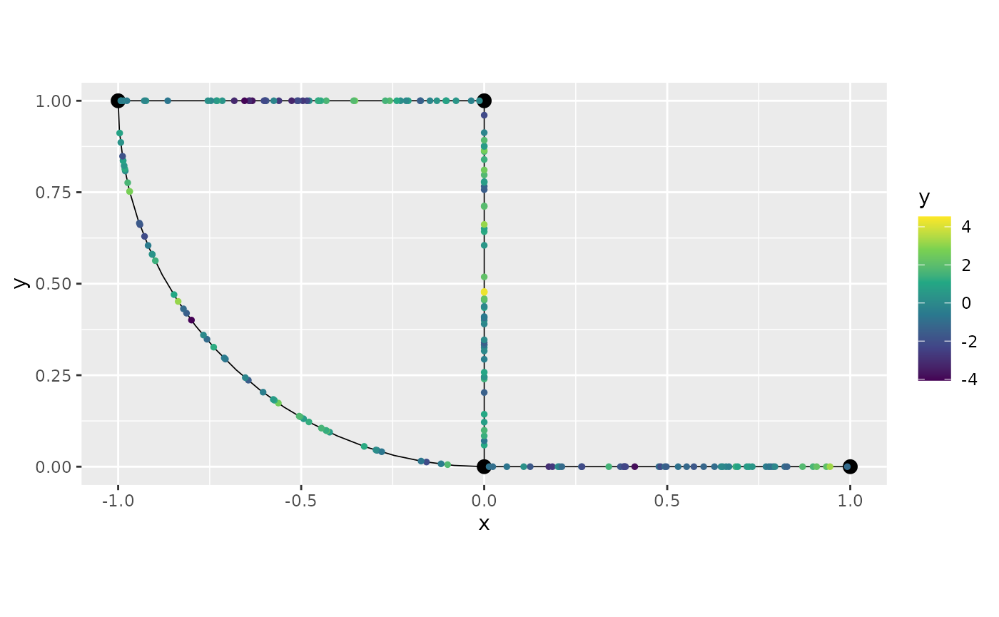

Now, we load the R-INLA package and create the inla model object with the graph_spde function. By default we have alpha=1.

library(INLA)
spde_model <- graph_spde(graph)

Now, we need to create the data object with the graph_data_spde() function, in which we need to provide a name for the random effect, which we will call field:

data_spde <- graph_data_spde(graph_spde = spde_model, name = "field")

The remaining is standard in R-INLA. We create the formula object and the inla.stack object with the inla.stack() function. The data needs to be in the graph (by using the add_observations() method) and should be supplied to the stack by the components of the data_spde list obtained from the graph_data_spde() function:

f.s <- y ~ -1 + Intercept + f(field, model = spde_model)

stk_dat <- inla.stack(data = data_spde[["data"]], 
                        A = data_spde[["basis"]], 
                        effects = c(
      data_spde[["index"]],
      list(Intercept = 1)
    ))

Now, we use the inla.stack.data() function:

data_stk <- inla.stack.data(stk_dat)

Finally, we fit the model:

spde_fit <- inla(f.s, data = data_stk, 
                  control.predictor=list(A=inla.stack.A(stk_dat)),
                               num.threads = "1:1")

Let us now obtain the estimates in the original scale by using the spde_metric_graph_result() function, then taking a summary():

spde_result <- spde_metric_graph_result(spde_fit, "field", spde_model)

summary(spde_result)

##            mean        sd 0.025quant  0.5quant 0.975quant      mode
## sigma 1.6495100 0.1332900  1.4059100 1.6429600    1.93198 1.6445800
## range 0.0864231 0.0170456  0.0584394 0.0844947    0.12515 0.0806159

We will now compare the means of the estimated values with the true values:

  result_df <- data.frame(
    parameter = c("std.dev", "range"),
    true = c(sigma, r),
    mean = c(
      spde_result$summary.sigma$mean,
      spde_result$summary.range$mean
    ),
    mode = c(
      spde_result$summary.sigma$mode,
      spde_result$summary.range$mode
    )
  )
  print(result_df)

##   parameter true       mean       mode
## 1   std.dev 2.00 1.64950919 1.64458457
## 2     range 0.15 0.08642314 0.08061591

We can also plot the posterior marginal densities with the help of the gg_df() function:

  posterior_df_fit <- gg_df(spde_result)

  library(ggplot2)

  ggplot(posterior_df_fit) + geom_line(aes(x = x, y = y)) + 
  facet_wrap(~parameter, scales = "free") + labs(y = "Density")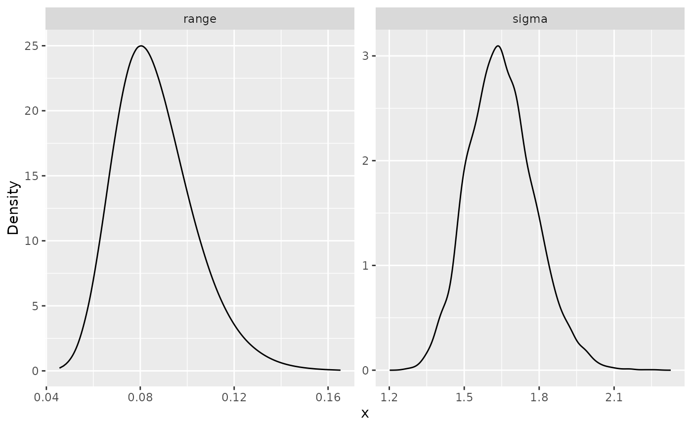

Kriging with our INLA implementation

Let us begin by obtaining an evenly spaced mesh with respect to the base graph:

obs_per_edge_prd <- 50
graph$build_mesh(n = obs_per_edge_prd)

Let us plot the resulting graph:

graph$plot(mesh=TRUE)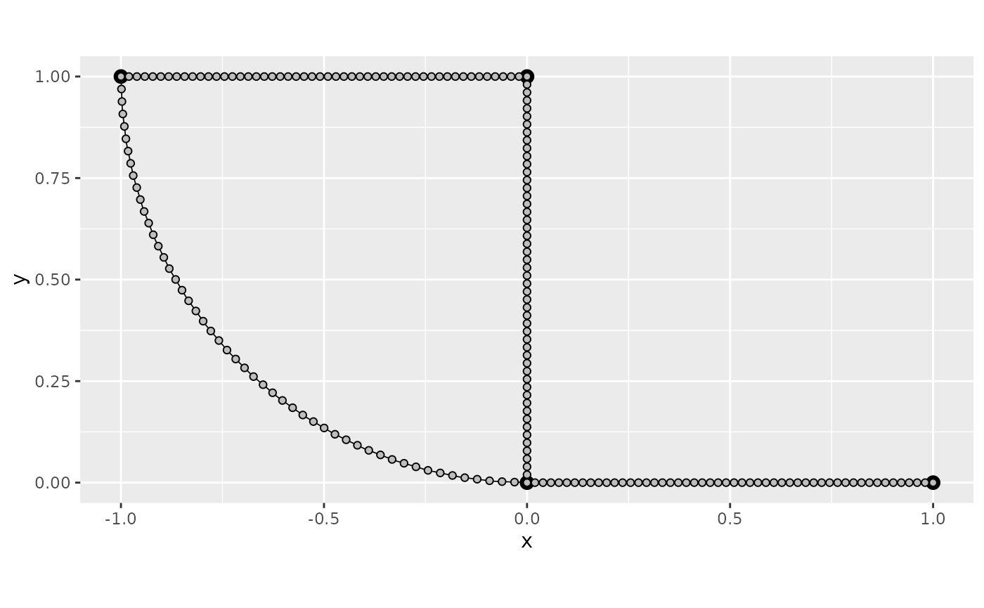

We will now add the observations on the mesh locations to the graph we fitted the R-INLA model. To this end we will use the add_mesh_observations() method. We will enter the response variables as NA. We can get the number of mesh nodes by counting the number of rows of the mesh$PtE attribute.

n_obs_mesh <- nrow(graph$mesh$PtE)
y_prd <- rep(NA, n_obs_mesh)
data_mesh <- data.frame(y = y_prd)
graph$add_mesh_observations(data = data_mesh)

## Adding observations...

## list()

We will now fit a new model with R-INLA with this new graph that contains the prediction locations. To this end, we create a new model object with the graph_spde() function:

spde_model_prd <- graph_spde(graph)

Now, let us create a new data object for prediction. Observe that we need to set drop_all_na to FALSE in order to not remove the prediction locations:

data_spde_prd <- graph_data_spde(spde_model_prd, drop_all_na = FALSE, name="field")

We will create a new vector of response variables, concatenating y to y_prd, then create a new formula object and the inla.stack object:

f_s_prd <- y ~ -1 + Intercept + f(field, model = spde_model_prd)

stk_dat_prd <- inla.stack(data = data_spde_prd[["data"]], 
                        A = data_spde_prd[["basis"]], 
                        effects = c(
      data_spde_prd[["index"]],
      list(Intercept = 1)
    ))

Now, we use the inla.stack.data() function and fit the model:

data_stk_prd <- inla.stack.data(stk_dat_prd)

spde_fit_prd <- inla(f_s_prd, data = data_stk_prd,
                               num.threads = "1:1")

We will now extract the means at the prediction locations:

idx_prd <- which(is.na(data_spde_prd[["data"]][["y"]]))

m_prd <- spde_fit_prd$summary.fitted.values$mean[idx_prd]

To improve visualization, we will plot the posterior means using the plot() method:

graph$plot_function(X = m_prd, vertex_size = 0, edge_width = 2)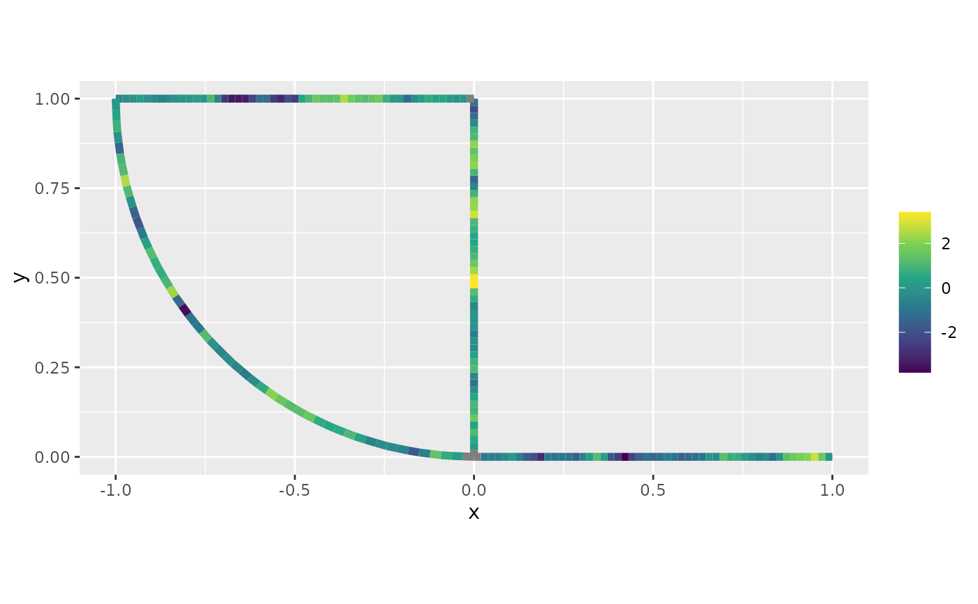

Finally, we can plot the predictions together with the data:

p <- graph$plot_function(X = m_prd, vertex_size = 0, edge_width = 1)
graph$plot(data="y", vertex_size = 0, data_size = 2, p = p, edge_width = 0)

An example with `alpha = 2`

We will now show an example where the parameter alpha is equal to 2. There is essentially no change in the commands above. Let us first clear the observations:

graph$clear_observations()

Let us now simulate the data with alpha=2. We will now sample in these observation locations and plot the latent field:

sigma <- 2
alpha <- 2
nu <- alpha - 0.5
r <- 0.15 # r stands for range


u <- sample_spde(range = r, sigma = sigma, alpha = alpha,
                 graph = graph, PtE = obs_loc)
graph$plot(X = u, X_loc = obs_loc)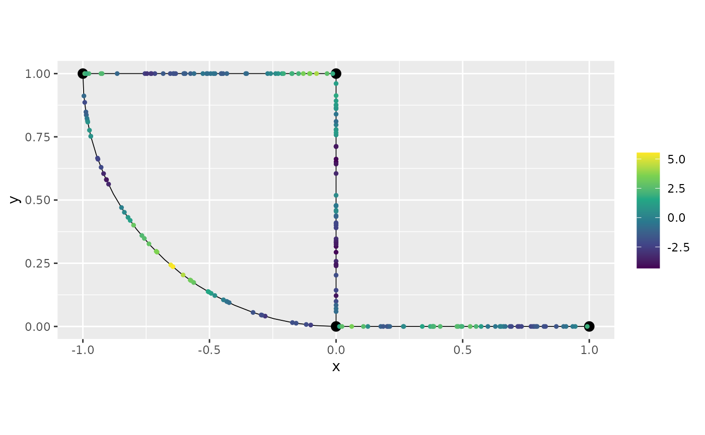

In the same way as before we will generate y and add the observations:

n_obs <- length(u)
sigma.e <- 0.1

y <- u + sigma.e * rnorm(n_obs)

df_graph <- data.frame(y = y, edge_number = obs_loc[,1],
                        distance_on_edge = obs_loc[,2])

graph$add_observations(data=df_graph, normalized=TRUE)

## list()

Let us now create the model object for alpha=2:

spde_model_alpha2 <- graph_spde(graph, alpha = 2)

Now, we will create the new data object with the graph_data_spde() function, in which we need to provide a name for the random effect, which we will call field:

data_spde_alpha2 <- graph_data_spde(graph_spde = spde_model_alpha2, 
                            name = "field")

We now proceed as before to prepare to fit the model:

f.s.2 <- y ~ -1 + Intercept + f(field, model = spde_model_alpha2)

stk_dat2 <- inla.stack(data = data_spde_alpha2[["data"]], 
                        A = data_spde_alpha2[["basis"]], 
                        effects = c(
      data_spde_alpha2[["index"]],
      list(Intercept = 1)
    ))

data_stk2 <- inla.stack.data(stk_dat2)

Finally, we fit the model:

spde_fit_alpha2 <- inla(f.s.2, data = data_stk2, 
          control.predictor=list(A=inla.stack.A(stk_dat2)),
                               num.threads = "1:1")

Let us now obtain the estimates in the original scale by using the spde_metric_graph_result() function, then taking a summary():

spde_result_alpha2 <- spde_metric_graph_result(spde_fit_alpha2, 
                            "field", spde_model_alpha2)

summary(spde_result_alpha2)

##           mean        sd 0.025quant 0.5quant 0.975quant     mode
## sigma 2.175780 0.2397420   1.749840 2.160380   2.687860 2.103500
## range 0.157442 0.0166731   0.127248 0.156589   0.192674 0.154826

We will now compare the means of the estimated values with the true values:

  result_df_alpha2 <- data.frame(
    parameter = c("std.dev", "range"),
    true = c(sigma, r),
    mean = c(
      spde_result_alpha2$summary.sigma$mean,
      spde_result_alpha2$summary.range$mean
    ),
    mode = c(
      spde_result_alpha2$summary.sigma$mode,
      spde_result_alpha2$summary.range$mode
    )
  )
  print(result_df_alpha2)

##   parameter true      mean      mode
## 1   std.dev 2.00 2.1757796 2.1034977
## 2     range 0.15 0.1574421 0.1548257

We can also plot the posterior marginal densities with the help of the gg_df() function:

  posterior_df_fit <- gg_df(spde_result_alpha2)

  library(ggplot2)

  ggplot(posterior_df_fit) + geom_line(aes(x = x, y = y)) + 
  facet_wrap(~parameter, scales = "free") + labs(y = "Density")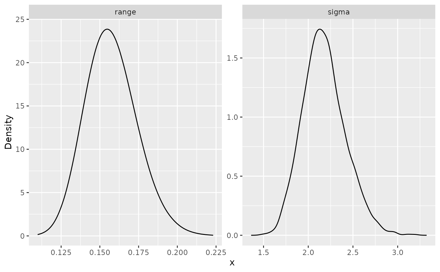

Fitting `R-INLA` models with replicates

We will now illustrate how to use our R-INLA implementation to fit models with replicates.

To simplify exposition, we will use the same base graph. So, we begin by clearing the observations.

graph$clear_observations()

We will use the same observation locations as for the previous cases. Let us sample 30 replicates:

sigma_rep <- 1.5
alpha_rep <- 1
nu_rep <- alpha_rep - 0.5
r_rep <- 0.2 # r stands for range
kappa_rep <- sqrt(8 * nu_rep) / r_rep

n_repl <- 30

u_rep <- sample_spde(range = r_rep, sigma = sigma_rep,
                 alpha = alpha_rep,
                 graph = graph, PtE = obs_loc,
                 nsim = n_repl)

Let us now generate the observed responses, which we will call y_rep.

n_obs_rep <- nrow(u_rep)
sigma_e <- 0.1

y_rep <- u_rep + sigma_e * matrix(rnorm(n_obs_rep * n_repl),
                                    ncol=n_repl)

The sample_spde() function returns a matrix in which each replicate is a column. We need to stack the columns together and a column to indicate the replicate:

dl_graph <- lapply(1:ncol(y_rep), function(i){data.frame(y = y_rep[,i],
                                          edge_number = obs_loc[,1],
                                          distance_on_edge = obs_loc[,2],
                                          repl = i)})
dl_graph <- do.call(rbind, dl_graph)

We can now add the the observations by setting the group argument to repl:

graph$add_observations(data = dl_graph, normalized=TRUE, 
                            group = "repl",
                            edge_number = "edge_number",
                            distance_on_edge = "distance_on_edge")

## Adding observations...

## list()

By definition the plot() method plots the first replicate. We can select the other replicates with the group argument. See the Working with metric graphs for more details.

graph$plot(data="y")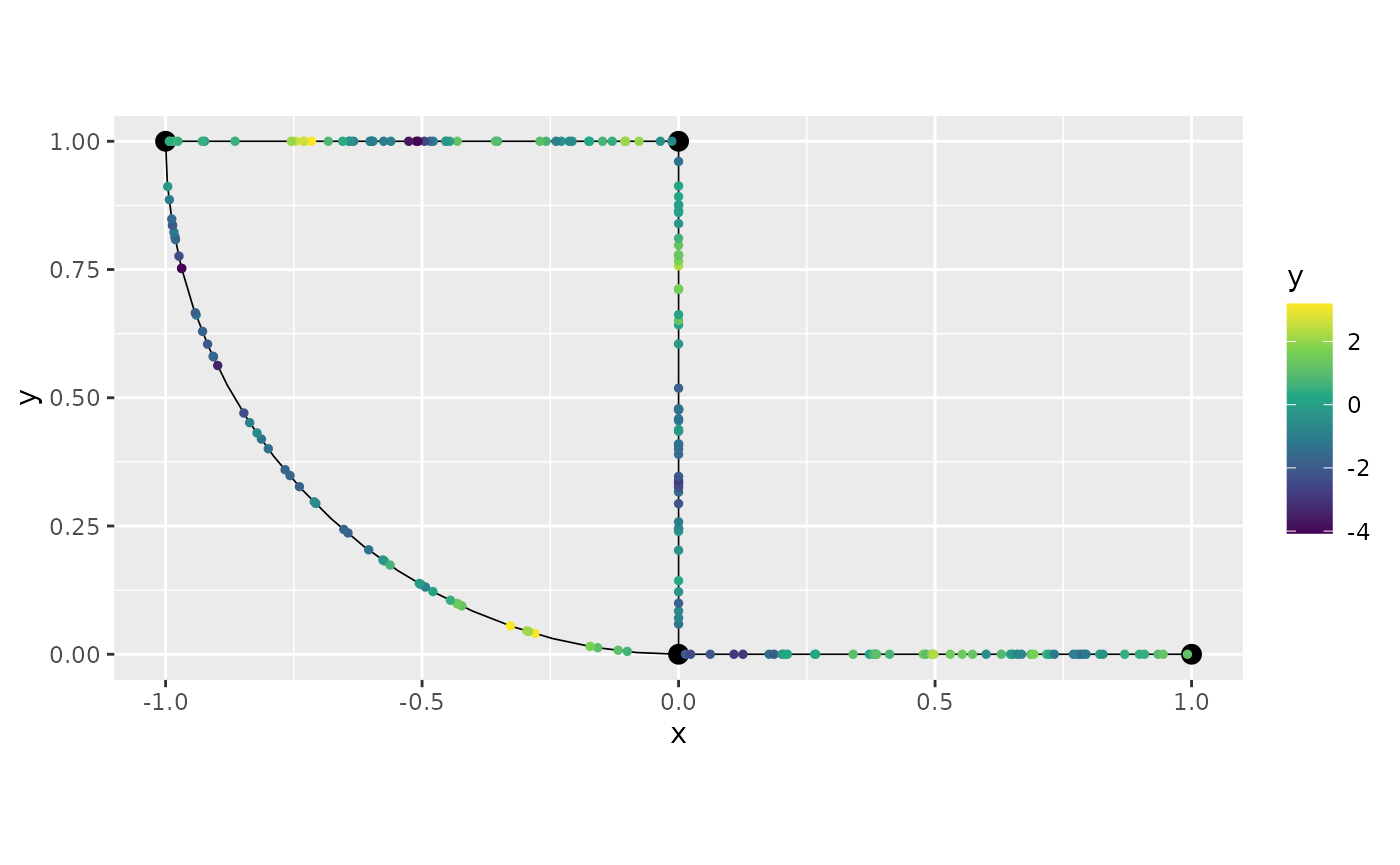

Let us plot another replicate:

graph$plot(data="y", group=2)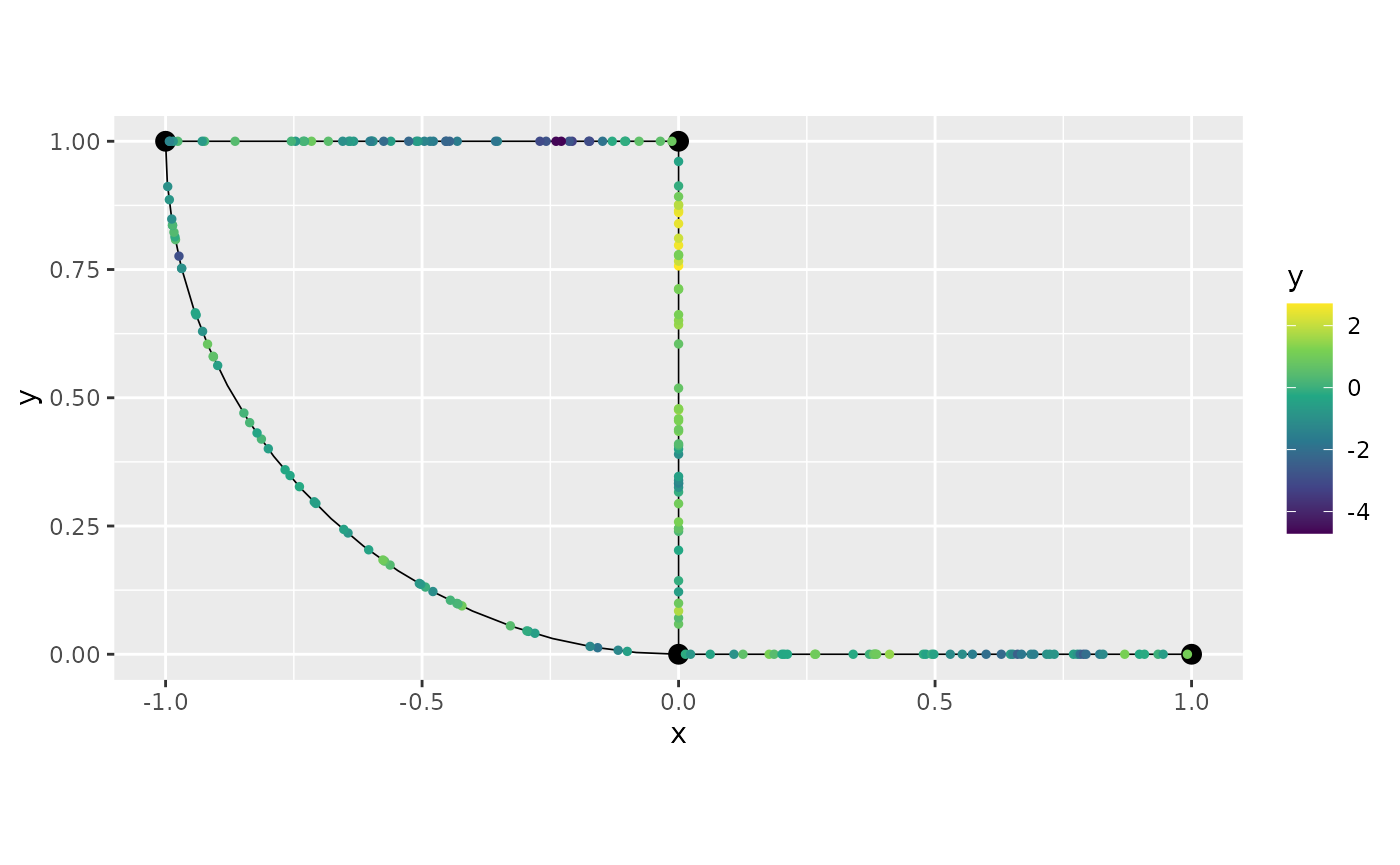

Let us now create the model object:

spde_model_rep <- graph_spde(graph)

Let us first consider a case in which we do not use all replicates. Then, we consider the case in which we use all replicates.

Thus, let us assume we want only to consider replicates 1, 3, 5, 7 and 9. To this end, we the index object by using the graph_data_spde() function with the argument repl set to the replicates we want, in this case c(1,3,5,7,9):

data_spde <- graph_data_spde(graph_spde=spde_model_rep,
                      name="field", repl = c(1,3,5,7,9), repl_col = "repl")

Next, we create the stack object, remembering that we need to input the components from data_spde:

stk_dat_rep <- inla.stack(data = data_spde[["data"]], 
                        A = data_spde[["basis"]], 
                        effects = c(
      data_spde[["index"]],
      list(Intercept = 1)
    ))

We now create the formula object, adding the name of the field (in our case field) attached with .repl a the replicate argument inside the f() function.

f_s_rep <- y ~ -1 + Intercept + 
    f(field, model = spde_model_rep, 
        replicate = field.repl)

Then, we create the stack object with The inla.stack.data() function:

data_stk_rep <- inla.stack.data(stk_dat_rep)

Now, we fit the model:

spde_fit_rep <- inla(f_s_rep, data = data_stk_rep, 
                control.predictor=list(A=inla.stack.A(stk_dat_rep)),
                               num.threads = "1:1")

Let us see the estimated values in the original scale:

spde_result_rep <- spde_metric_graph_result(spde_fit_rep, 
                        "field", spde_model_rep)

summary(spde_result_rep)

##           mean        sd 0.025quant 0.5quant 0.975quant     mode
## sigma 1.608640 0.0844529   1.445240 1.607040   1.775820 1.602970
## range 0.225623 0.0265312   0.176931 0.224417   0.280786 0.222684

Let us compare with the true values:

  result_df_rep <- data.frame(
    parameter = c("std.dev", "range"),
    true = c(sigma_rep, r_rep),
    mean = c(
      spde_result_rep$summary.sigma$mean,
      spde_result_rep$summary.range$mean
    ),
    mode = c(
      spde_result_rep$summary.sigma$mode,
      spde_result_rep$summary.range$mode
    )
  )
  print(result_df_rep)

##   parameter true      mean      mode
## 1   std.dev  1.5 1.6086418 1.6029748
## 2     range  0.2 0.2256235 0.2226845

Now, let us consider the case with all replicates. We create a new data object by using the graph_data_spde() function with the argument repl set to .all:

data_spde_rep <- graph_data_spde(graph_spde=spde_model_rep, 
                    name="field", 
                    repl = ".all", repl_col = "repl")

Now the stack:

stk_dat_rep <- inla.stack(data = data_spde_rep[["data"]], 
                        A = data_spde_rep[["basis"]], 
                        effects = c(
      data_spde_rep[["index"]],
      list(Intercept = 1)
    ))

We now create the formula object in the same way as before:

f_s_rep <- y ~ -1 + Intercept + 
    f(field, model = spde_model_rep, 
        replicate = field.repl)

Then, we create the stack object with The inla.stack.data() function:

data_stk_rep <- inla.stack.data(stk_dat_rep)

Now, we fit the model:

spde_fit_rep <- inla(f_s_rep, data = data_stk_rep,
                               num.threads = "1:1")

Let us see the estimated values in the original scale:

spde_result_rep <- spde_metric_graph_result(spde_fit_rep, 
                        "field", spde_model_rep)

summary(spde_result_rep)

##           mean        sd 0.025quant 0.5quant 0.975quant     mode
## sigma 1.527030 0.0329779   1.464300 1.526420   1.593920 1.527310
## range 0.222953 0.0105895   0.202875 0.222686   0.244477 0.222159

Let us compare with the true values:

  result_df_rep <- data.frame(
    parameter = c("std.dev", "range"),
    true = c(sigma_rep, r_rep),
    mean = c(
      spde_result_rep$summary.sigma$mean,
      spde_result_rep$summary.range$mean
    ),
    mode = c(
      spde_result_rep$summary.sigma$mode,
      spde_result_rep$summary.range$mode
    )
  )
  print(result_df_rep)

##   parameter true     mean      mode
## 1   std.dev  1.5 1.527034 1.5273119
## 2     range  0.2 0.222953 0.2221589

Bolin, David, Alexandre B. Simas, and Jonas Wallin. 2023. “Statistical Properties of Gaussian Whittle–Matérn Fields on Metric Graphs.” arXiv:2304.10372.

———. 2024. “Gaussian Whittle–Matérn Fields on Metric Graphs.” Bernoulli 30: 1611–39.

David Bolin, Alexandre B. Simas, and Jonas Wallin

Created: 2022-11-23. Last modified: 2024-12-13.

Introduction

A toy dataset

`R-INLA` implementation

Kriging with our INLA implementation

An example with `alpha = 2`

Fitting `R-INLA` models with replicates

INLA interface for Whittle--Matérn fields on metric graphs

David Bolin, Alexandre B. Simas, and Jonas Wallin

Created: 2022-11-23. Last modified: 2024-12-13.

Introduction

A toy dataset

R-INLA implementation

Kriging with our INLA implementation

An example with alpha = 2

Fitting R-INLA models with replicates

`R-INLA` implementation

An example with `alpha = 2`

Fitting `R-INLA` models with replicates