MetricGraph: Random Fields on Metric Graphs

David Bolin, Alexandre B. Simas, and Jonas Wallin

Created: 2022-11-26. Last modified: 2025-05-21.

Introduction

There has lately been much interest in statistical modeling of data on compact metric graphs such as street or river networks based on Gaussian random fields.

The R package MetricGraph contains functions for working with data and random fields on compact metric graphs. The main functionality is contained in the metric_graph class, which is used for specifying metric graphs, adding data to them, visualization, and other basic functions that are needed for working with data and random fields on metric graphs. The package also implements three types of Gaussian processes on metric graphs: The Whittle–Matérn fields introduced by Bolin, Simas, and Wallin (2024) and Bolin, Simas, and Wallin (2023), Gaussian processes with isotropic covariance functions Anderes, Møller, and Rasmussen (2020), and Gaussian models based on the graph Laplacian Borovitskiy et al. (2021).

Basic statistical tasks such as likelihood evaluation and prediction is implemented for these three types of models in MetricGraph. Further, the package also contains interfaces to R-INLA Lindgren and Rue (2015), package available from http://R-INLA. org/download/ and inlabru Bachl et al. (2019) that facilitates using those packages for full Bayesian inference of general Latent Gaussian Models (LGMs) that includes Whittle–Matérn fields on metric graphs.

The package is available to install via the repository https://github.com/davidbolin/MetricGraph.

The following sections describe the main functionality of the package and summarizes some of the required theory. Section 2 introduces metric graphs and the metric_graph class, Section 3 shows how to work with random fields on metric graphs, and Section 4 introduces the inlabru interface of the package through an application to real data. For a complete introduction to the functionality of the package, we refer to the Vignettes available on the package homepage https://davidbolin.github.io/MetricGraph/. In particular, that contains an introduction to the INLA interface, the implementation of Whittle–Matérn fields with general smoothness, and further details and examples for all methods in the package.

The metric_graph class

A compact metric graph $\Gamma$ consists of a set of finitely many vertices $\mathcal{V}=\{v_i\}$ and a finite set $\mathcal{E}=\{e_j\}$ of edges connecting the vertices. Each edge $e$ is defined by a pair of vertices $(v_i,v_k)$ and a finite length $l_e \in (0,\infty)$. An edge in the graph is a curve parametrized by arc-length, and a location $s\in \Gamma$ is a position on an edge, and can thus be represented as a touple $(e,t)$ where $t\in[0,l_e]$.

Basic constructions

A metric graph is represented in the MetricGraph package through the class metric_graph. An object of this class can be constructed in two ways. The first is to specify the vertex matrix V and the edge matrix E, and it is then assumed that all edges are straight lines. The second, more flexible, option is to specify the object from a SpatialLines object using the sp package (Bivand, Pebesma, and Gomez-Rubio 2013).

To illustrate this, we use the osmdata package to download data from OpenStreetMap. In the following code, we extract the streets on the campus of King Abdullah University of Science and Technology (KAUST) as a SpatialLines object:

call <- opq(bbox = c(39.0884, 22.33, 39.115, 22.3056))
call <- add_osm_feature(call, key = "highway",value=c("motorway",
                                                      "primary","secondary",
                                                      "tertiary",
                                                      "residential"))
data <- osmdata_sf(call)

We can now create the metric graph as follows.

graph <- metric_graph$new(data)
graph$plot(vertex_size = 0.5)

Let us also build an interactive plot with the underlying map:

graph$plot(vertex_size = 0.5, type = "mapview")

Observe that when we create this graph from osmdata, it also includes the edge data as edge weights:

graph$get_edge_weights()

## # A tibble: 368 × 11
##    osm_id   name    bridge highway layer lit   maxspeed maxweight oneway surface
##    <chr>    <chr>   <chr>  <chr>   <chr> <chr> <chr>    <chr>     <chr>  <chr>  
##  1 38085402 Discov… NA     reside… NA    yes   40       NA        NA     NA     
##  2 38085409 King A… NA     primary NA    yes   60       NA        yes    NA     
##  3 39425304 King A… NA     primary NA    NA    20       NA        yes    NA     
##  4 39425484 Peace … NA     reside… NA    NA    40       NA        NA     NA     
##  5 39425550 Island… NA     reside… NA    NA    40       NA        NA     NA     
##  6 39425743 Coral … NA     reside… NA    yes   40       NA        NA     NA     
##  7 39425802 Hammou… NA     reside… NA    yes   40       NA        NA     NA     
##  8 39426595 Najel … NA     reside… NA    yes   40       NA        yes    NA     
##  9 39478848 Discov… NA     reside… NA    NA    40       NA        NA     NA     
## 10 39478849 Explor… NA     reside… NA    yes   40       NA        NA     NA     
## # ℹ 358 more rows
## # ℹ 1 more variable: .weights <dbl>

Now, note that when creating the graph there was a warning saying that the graph is not connected, so let us create a graph_components object that contains all connected components as graphs and then extract the largest connected component to work with

graphs <- graph_components$new(edges = data)
graph <- graphs$get_largest()
graph$plot(vertex_size = 0)

Here is the interactive plot:

graph$plot(vertex_size = 0, type = "mapview")

The graph object now contains all important features of the graph, such as the vertex matrix graph$V, the number of vertices graph$nV, the edge matrix graph$E, the number of edges graph$nE, and the vector of all edge lengths graph$get_edge_lengths() given in the unit km. Thus, we can obtain the range of the edge lengths in the unit m as:

range(graph$get_edge_lengths(unit="m")) 

## Units: [m]
## [1]    7.120828 1674.529905

Observe that it also contains the corresponding edge weights:

graph$get_edge_weights()

## # A tibble: 317 × 11
##    osm_id   name    bridge highway layer lit   maxspeed maxweight oneway surface
##    <chr>    <chr>   <chr>  <chr>   <chr> <chr> <chr>    <chr>     <chr>  <chr>  
##  1 38085402 Discov… NA     reside… NA    yes   40       NA        NA     NA     
##  2 38085409 King A… NA     primary NA    yes   60       NA        yes    NA     
##  3 39425304 King A… NA     primary NA    NA    20       NA        yes    NA     
##  4 39425484 Peace … NA     reside… NA    NA    40       NA        NA     NA     
##  5 39425550 Island… NA     reside… NA    NA    40       NA        NA     NA     
##  6 39425743 Coral … NA     reside… NA    yes   40       NA        NA     NA     
##  7 39426595 Najel … NA     reside… NA    yes   40       NA        yes    NA     
##  8 39478848 Discov… NA     reside… NA    NA    40       NA        NA     NA     
##  9 39478849 Explor… NA     reside… NA    yes   40       NA        NA     NA     
## 10 39478852 Transf… NA     reside… NA    NA    40       NA        NA     NA     
## # ℹ 307 more rows
## # ℹ 1 more variable: .weights <dbl>

We will also remove the vertices of degree 2 by using the prune_vertices() method:

graph$prune_vertices()
graph$plot()

Observe that no vertex of degree 2 was pruned. This means that the edge weights are different. If one wants to prune regardless of losing information from the edge weights, one can simply set the argument check_weights to FALSE in the prune_vertices() method:

graph$prune_vertices(check_weights=FALSE)
graph$plot()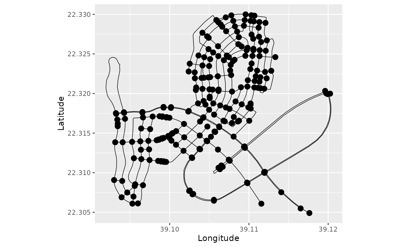

However, note that a warning was given due to incompatible edge weights.

Understanding coordinates on graphs

The locations of the vertices are specified in Euclidean coordinates. However, when specifying a position on the graph, it is not practical to work with Euclidean coordinates since not all locations in Euclidean space are locations on the graph. It is instead better to specify a location on the graph by the touple $(i, t)$, where $i$ denotes the number of the edge and $t$ is the location on the edge. The location $t$ can either be specified as the distance from the start of the edge (and then takes values between 0 and the length of the edge) or as the normalized distance from the start of the edge (and then takes values between 0 and 1). The function coordinates can be used to convert between coordinates in Euclidean space and locations on the graph. For example the location at normalized distance 0.2 from the start of the second edge is:

graph$coordinates(PtE = matrix(c(2, 0.2), 1,2), normalized = TRUE)

##          [,1]     [,2]
## [1,] 39.11693 22.31903

The function can also be used to find the closest location on the graph for a location in Euclidean space:

graph$coordinates(XY = matrix(c(39.117, 22.319), 1,2))

##      [,1]      [,2]
## [1,]    2 0.1967297

In this case, the normalized argument decides whether the returned value should be given in normalized distance or not.

Adding data to the graph

Given that we have constructed the metric graph, we can now add data to it. For further details on data manipulation on metric graphs, see Data manipulation on metric graphs. As an example, let us sample some locations on edges at random and add data to them in the graph:

n.obs <- 10
data <- data.frame(edge_number = sample(1:graph$nE, n.obs, replace=TRUE),
                   distance_on_edge = runif(n.obs),
                   y = rnorm(n.obs))
graph$add_observations(data = data, normalized = TRUE)

## Adding observations...

## Assuming the observations are normalized by the length of the edge.

## The unit for edge lengths is km

## The current tolerance for removing distant observations is (in km): 0.837264952278885

graph$plot(data = "y", vertex_size = 0, type = "mapview")

## Warning: Found more unique colors (100) than unique zcol values (10)! 
## Trimming color vector to match number of zcol values.

One should note here that one needs to specify normalized = TRUE in the function to specify that the locations are in normalized distance on the edges. If this command is not set, the distances are interpreted as not being normalized. The add_observations() function accepts multiple types of inputs. One scenario that can be common in applications is to have the data as SpatialPoints objects, and one can then add the observations as a SpatialPointsDataFrame. To illustrate this, let us again sample some locations at random on the graph, then use the function coordinates to transform those to Longitude Latitude coordinates, which we then use to create a SpatialPointsDataFrame object which we add to the graph:

obs.loc <- cbind(sample(1:graph$nE, n.obs, replace=TRUE), runif(n.obs))
obs.lonlat <- graph$coordinates(PtE = obs.loc, normalized = TRUE)
obs <- rnorm(n.obs)
points <- SpatialPointsDataFrame(coords = obs.lonlat,
                                 data = data.frame(y = obs))
graph$add_observations(points)

## Adding observations...

## The unit for edge lengths is km

## The current tolerance for removing distant observations is (in km): 0.837264952278885

## Converting data to PtE

## This step may take long. If this step is taking too long consider pruning the vertices to possibly obtain some speed up.

## $removed
## [1] y        .coord_x .coord_y
## <0 rows> (or 0-length row.names)

graph$plot(data = "y", vertex_size = 0, type = "mapview")

If we want to replace the data in the object, we can use clear_observations() to remove all current data.

Working with functions on metric graphs

When working with data on metric graphs, one often wants to display functions on the graph. The best way to visualize functions on the graph is to evaluate them on a fine mesh over the graph and then use plot_function. To illustrate this procedure, let us construct a mesh on the graph:

graph$build_mesh(h = 100/1000)
graph$plot(mesh=TRUE, type = "mapview")

## Warning in cbind(`Feature ID` = fid, mat): number of rows of result is not a
## multiple of vector length (arg 1)

In the command build_mesh, the argument h decides the largest spacing between nodes in the mesh. Above we chose that as 100m which is a bit coarse. So let us reduce the value of h to 10m and rebuild the mesh:

  graph$build_mesh(h = 10/1000)

Suppose now that we want to display the function $f(s) = \text{Longitude}(s) - \text{Latitude}(s)$ on this graph. We then first evaluate it on the vertices of the mesh and then use the function plot_function to display it:

lon <- graph$mesh$V[, 1]
lat <- graph$mesh$V[, 2]
f <- lon - lat
graph$plot_function(X = f, vertex_size = 0, edge_width = 0.5,
                type = "mapview")

Alternatively, we can set type = "plotly" in the plot command to get a 3D visualization of the function by using the plotly (Sievert 2020) package. When the first argument of plot_function is a vector, the function assumes that the values in the vector are the values of the function evaluated at the vertices of the mesh. As an alternative, one can also provide the first argument as a matrix consisting of the triplets $(i, t, f(i, t))$, where $i$ denotes the edge number, $t$ the location on the edge, and $f(i, t)$ the value at that point.

Random fields on metric graphs

Having defined the metric graph, we are now ready to specify Gaussian processes on it. In this section, we will briefly cover the three main types of Gaussian processes that are supported. Be begin by the main class of models, the Whittle–Matérn fields, then consider Gaussian processes with isotropic covariance functions, and finally look at discrete models based on the graph Laplacian.

Whittle–Matérn fields

The Gaussian Whittle–Matérn fields are specified as solutions to the stochastic differential equation $$(\kappa^2 - \Delta)^{\alpha/2} \tau u = \mathcal{W}$$ on the metric graph $\Gamma$. We can work with these models without and approximations if the smoothness parameter $\alpha$ is an integer, and this is what we focus on in this vignette. For details on the case of a general smoothness parameter, see Whittle–Matérn fields with general smoothness.

Sampling

As an example, let us simulate the field $u$ on the graph using $\alpha = 1$. To do so, we again draw some locations at random, then sample the field at these locations and plot the result

sigma <- 1.3
range <- 0.15 # range parameter
sigma_e <- 0.1

n.obs <- 200
obs.loc <- cbind(sample(1:graph$nE, n.obs, replace=TRUE), runif(n.obs))

u <- sample_spde(range = range, sigma = sigma, alpha = 1,
                 graph = graph, PtE = obs.loc)
graph$clear_observations()
graph$add_observations(data = data.frame(edge_number = obs.loc[, 1],
                                         distance_on_edge = obs.loc[, 2],
                                         u = u),
                       normalized = TRUE)

## Adding observations...

## Assuming the observations are normalized by the length of the edge.

## The unit for edge lengths is km

## The current tolerance for removing distant observations is (in km): 0.837264952278885

graph$plot(data = "u", vertex_size = 0, type = "mapview")

We can also plot the interactive version:

graph$plot(data = "u", vertex_size = 0, type = "mapview")

We can also sample the field at the mesh on the graph as follows:

u <- sample_spde(range = range, sigma = sigma, alpha = 1,
                 graph = graph, type = "mesh")
graph$plot_function(X = u, vertex_size = 0, edge_width = 0.5,
            type = "mapview")

Since $\alpha=1$, these sample paths are continuous but not differentiable. To visualize the correlation structure of the field, we can compute and plot the covariances between some point and all other points in the graph as follows:

C <- spde_covariance(c(200, 0.1), range = range, sigma = sigma, alpha = 1,
                            graph = graph)
graph$plot_function(X = C, vertex_size = 0, edge_width = 0.5,
            type = "mapview")

To obtain a field with differentiable sample paths, we can change to $\alpha=2$ in the code above.

Inference

In the following examples we will consider models without replicates. Please, see the Gaussian random fields on metric graphs vignette for examples with replicates.

Suppose that we have data of the form $$y_i = \beta_1\text{lon}(s_i) + \beta_1\text{lat}(s_i) + u(s_i) + \varepsilon_i, \quad i=1,\ldots,n$$ where $s_i\in \Gamma$ are observation locations, lon and lat are the longitude and latitude of these locations, $\beta_1,\beta_2$ are some regression coefficients, and $\varepsilon_i$ are independent centered Gaussian variables $N(0,\sigma_e^2)$ representing measurement noise.

Let us create such observations, clear the current data in the graph, and finally add the data on the graph:

sigma <- 2
range <- 0.2 # range parameter
sigma_e <- 0.1

n.obs.1 <- 400 # all edges
n.obs.2 <- 100 # long edges

n.obs <- n.obs.1 + n.obs.2

obs.loc <- cbind(sample(1:graph$nE, n.obs.1, replace=TRUE), runif(n.obs.1))

# Let us now add some locations on long edges:
long.edges <- graph$edge_lengths > 0.5

obs.loc <- rbind(obs.loc, cbind(sample(which(long.edges), n.obs.2, replace=TRUE), runif(n.obs.2)))

u <- sample_spde(range = range, sigma = sigma, alpha = 1,
                 graph = graph, PtE = obs.loc)

beta0 = -1
beta1 = 1
beta2 = 2
lonlat <- graph$coordinates(PtE = obs.loc)
scaled_lonlat <- scale(lonlat)
y <- beta0 + beta1 * scaled_lonlat[, 1] + beta2 * scaled_lonlat[, 2] + u + sigma_e*rnorm(n.obs)

data <- data.frame(edge_number = obs.loc[, 1],
                   distance_on_edge = obs.loc[, 2],
                   lon = scaled_lonlat[, 1],
                   lat = scaled_lonlat[, 2],
                   y = y)

graph$clear_observations()
graph$plot(X = y, X_loc = obs.loc, vertex_size = 0, type = "mapview")

graph$add_observations(data = data, normalized = TRUE)

## Adding observations...

## Assuming the observations are normalized by the length of the edge.

## The unit for edge lengths is km

## The current tolerance for removing distant observations is (in km): 0.837264952278885

Our goal now is to fit a linear mixed-effects model on this data assuming a Whittle-Mat'ern latent model with $\alpha=1$. To this end, we can use the graph_lme() function.

If we do not specify the model, it will fit a linear regression model. So, let us first fit a simple linear regression model to illustrate:

res_lm <- graph_lme(y ~ lon + lat, graph = graph)

We can get the summary:

summary(res_lm)

## 
## Linear regression model
## 
## Call:
## graph_lme(formula = y ~ lon + lat, graph = graph)
## 
## Fixed effects:
##             Estimate Std. Error t value Pr(>|t|)    
## (Intercept) -0.89407    0.07667  -11.66   <2e-16 ***
## lon          1.09752    0.08044   13.64   <2e-16 ***
## lat          2.09277    0.08044   26.02   <2e-16 ***

## 
## No random effects.

## 
## Measurement error:
## std. dev 
## 1.714391 
## ---
## Signif. codes:  0 '***' 0.001 '**' 0.01 '*' 0.05 '.' 0.1 ' ' 1 
## 
## Log-Likelihood:  -977.4937

Let us now fit the linear mixed-effects model with a Whittle-Mat'ern latent model with $\alpha=1$. To this end, we can either specify the model argument as 'alpha1' or as the following list: list(type = 'WhittleMatern', alpha = 1). The list makes it easier to understand which model is being chosen as a random effect, however, it makes it longer, and less convenient, to write. Let us use the simplified form:

res <- graph_lme(y ~ lon + lat, graph = graph, model = 'WM1')

Let us get the summary of the result:

summary(res)

## 
## Latent model - Whittle-Matern with alpha = 1
## 
## Call:
## graph_lme(formula = y ~ lon + lat, graph = graph, model = "WM1")
## 
## Fixed effects:
##             Estimate Std.error z-value Pr(>|z|)    
## (Intercept)  -0.9048    0.1379  -6.560 5.40e-11 ***
## lon           1.0062    0.1371   7.341 2.12e-13 ***
## lat           2.0877    0.1419  14.717  < 2e-16 ***
## 
## Random effects:
##       Estimate Std.error z-value
## tau   0.112763  0.004769  23.645
## kappa 9.823977  1.338642   7.339
## 
## Random effects (Matern parameterization):
##       Estimate Std.error z-value
## sigma  2.00066   0.10206  19.604
## range  0.20358   0.02773   7.343
## 
## Measurement error:
##           Estimate Std.error z-value
## std. dev 0.0002638 0.0569199   0.005
## ---
## Signif. codes:  0 '***' 0.001 '**' 0.01 '*' 0.05 '.' 0.1 ' ' 1 
## 
## Log-Likelihood:  -840.8517 
## Number of function calls by 'optim' = 47
## Optimization method used in 'optim' = L-BFGS-B
## 
## Time used to:     fit the model =  10.67438 secs

We can obtain additional information by using glance():

glance(res)

## # A tibble: 1 × 9
##    nobs    sigma logLik   AIC   BIC deviance df.residual model         alpha
##   <int>    <dbl>  <dbl> <dbl> <dbl>    <dbl>       <dbl> <chr>         <dbl>
## 1   500 0.000264  -841. 1694. 1719.    1682.         494 WhittleMatern     1

We will now compare with the true values of the random effects:

sigma_e_est <- res$coeff$measurement_error[[1]]
sigma_est <- res$matern_coeff$random_effects[1]
range_est <- res$matern_coeff$random_effects[2]
results <- data.frame(sigma_e = c(sigma_e, sigma_e_est),
                      sigma = c(sigma, sigma_est),
                      range = c(range, range_est),
                      row.names = c("Truth", "Estimate"))
print(results)

##               sigma_e    sigma     range
## Truth    0.1000000000 2.000000 0.2000000
## Estimate 0.0002638459 2.000662 0.2035835

Given these estimated parameters, we can now do kriging to estimate the field at locations in the graph. As an example, we now obtain predictions on the regular mesh that we previously constructed. First, we obtain the covariates on the mesh locations.

Now, we can compute the predictions for $y$. First, let us compute the posterior mean for the field at the observation locations and plot the residuals between the posterior means and the field:

pred_u <- predict(res, newdata = data, normalized = TRUE)
pred_u$resid_field <- pred_u$re_mean - u
pred_u <- graph$process_data(data = pred_u, normalized=TRUE)
pred_u %>% graph$plot(data = "resid_field", vertex_size = 0,
            type = "mapview")

We can also obtain predictions by using the augment() function:

Let us first plot the predictions for the field, then the fitted values:

pred_aug <- augment(res, newdata = data, normalized = TRUE)

pred_aug %>% graph$plot(data = ".random", vertex_size = 0,
            type = "mapview")

Let us now plot the fitted values along with the observed values:

pred_aug %>% graph$plot(data = ".fitted", vertex_size = 0,
            type = "mapview")

Let us now obtain predictions of the field on a mesh of equally spaced nodes on the graph. First, let us create the mesh and data.frame:

graph$build_mesh(h = 50/1000)
lonlat_mesh <- graph$coordinates(PtE = graph$mesh$VtE)
scaled_lonlat_mesh <- scale(lonlat_mesh, 
                            center = attr(scaled_lonlat, "scaled:center"),
                            attr(scaled_lonlat, "scaled:scale"))
data_mesh_pred <- data.frame(lon = scaled_lonlat_mesh[,1],
                              lat = scaled_lonlat_mesh[,2],
                              edge_number = graph$mesh$VtE[,1],
                              distance_on_edge = graph$mesh$VtE[,2])
# Let us remove duplicated vertices (that were created due to being too close)
data_mesh_pred <- data_mesh_pred[!duplicated(graph$mesh$V),]

Now, let us obtain the predictions. We can obtain estimates for the latent field by taking the re_mean element from the pred list obtained by calling prediction():

pred <- predict(res, newdata=data_mesh_pred, normalized=TRUE)
u_est <- pred$re_mean
graph$plot_function(X = u_est, vertex_size = 0, edge_width = 0.5,
            type = "mapview")

Finally, let us obtain predictions for the observed values on the mesh. In this case we use the mean component of the pred list:

y_est <- pred$mean
graph$plot_function(X = y_est, vertex_size = 0, edge_width = 0.5,
            type = "mapview")

The same procedure can be done with $\alpha = 2$. One can also estimate $\alpha$ from data as described in the vignette Whittle–Matérn fields with general smoothness.

Isotropic Gaussian fields

For metric graphs with Euclidean edges, Anderes, Møller, and Rasmussen (2020) showed that one can define valid Gaussian processes through various isotropic covariance functions if the distances between points are measured in the so-called resistance metric $d(\cdot,\cdot)$. One example of a valid covariance function is the isotropic exponential covariance function $$r(d(s,t)) = \sigma^2\exp(-\kappa d(s,t)).$$ This covariance is very similar to that of the Whittle–Mat'ern fields with $\alpha = 1$. Between the two, we recommend using the Whittle–Matérn model since it has Markov properties which makes inference much faster. Further, that covariance is well-defined for any compact metric graph, whereas the isotropic exponential is only guaranteed to be positive definite if the graph has Euclidean edges. See Bolin, Simas, and Wallin (2023) for further comparisons.

However, let us now illustrate how to use it for the data that we generated above. To work with the covariance function, the only cumbersome thing is to compute the metric. The metric_graph class has built in support for this, and we can obtain the distances between the observation locations as

graph$compute_resdist()

However, if the goal is to fit a model using this covariance function, there is no need for the user to compute it. It is done internally when one uses the graph_lme() function. We need to set the model argument in graph_lme() as a list with type "isoCov" (there is no need to add additional arguments, as the exponential covariance is the default). Let us fit a linear regression model with a random effect given by a Gaussian field with an isotropic exponential covariance function (alternatively, one can also write model = 'isoExp'):

res_exp <- graph_lme(y ~ lon + lat, graph = graph, model = list(type = "isoCov"))

## Warning in graph_lme(y ~ lon + lat, graph = graph, model = list(type =
## "isoCov")): No check for Euclidean edges have been perfomed on this graph. The
## isotropic covariance models are only known to work for graphs with Euclidean
## edges. You can check if the graph has Euclidean edges by running the
## `check_euclidean()` method. See the vignette
## https://davidbolin.github.io/MetricGraph/articles/isotropic_noneuclidean.html
## for further details.

Observe that we received a warning saying that we did not check if the graph has Euclidean edges. This is due to the fact that the isotropic covariance models are only known to work for graphs with Euclidean edges. Let us check if the graph has Euclidean edges. To this end, we need to use the check_euclidean() method:

graph$check_euclidean()

Now, we simply call the graph to print its characteristics to check the information:

graph

## A metric graph with  183  vertices and  269  edges.
## 
## Vertices:
##   Degree 1: 37;  Degree 2: 2;  Degree 3: 83;  Degree 4: 57;  Degree 5: 4; 
##   With incompatible directions:  2 
## 
## Edges: 
##   Lengths: 
##       Min: 0.009307252  ; Max: 1.67453  ; Total: 57.17622 
##   Weights: 
##       Columns: osm_id name bridge highway layer lit maxspeed maxweight oneway surface .weights 
##   That are circles:  0 
## 
## Graph units: 
##   Vertices unit:  degree  ; Lengths unit:  km 
## 
## Longitude and Latitude coordinates:  TRUE
##   Which spatial package:  sp 
##   CRS:  +proj=longlat +datum=WGS84 +no_defs
## 
## Some characteristics of the graph:
##   Connected: TRUE
##   Has loops: FALSE
##   Has multiple edges: TRUE
##   Is a tree: FALSE
##   Distance consistent: unknown

## To check if the graph satisfies the distance consistency, run the `check_distance_consistency()` method.

##   Has Euclidean edges: FALSE

Observe that this graph DOES NOT have Euclidean edges. This means that the model with isotropic exponential covariance is not guaranteed to work for this graph. In any case, we can try to fit it anyway. Observe that we will now receive a different warning, since now we know for fact that the graph does not have Euclidean edges. In this case, we will set model to isoexp for conveniency.

res_exp <- graph_lme(y ~ lon + lat, graph = graph, model = "isoexp")

## Warning in graph_lme(y ~ lon + lat, graph = graph, model = "isoexp"): This
## graph DOES NOT have Euclidean edges. The isotropic covariance models are NOT
## guaranteed to work for this graph! See the vignette
## https://davidbolin.github.io/MetricGraph/articles/isotropic_noneuclidean.html
## for further details.

summary(res_exp)

## 
## Latent model - Covariance-based model
## 
## Call:
## graph_lme(formula = y ~ lon + lat, graph = graph, model = "isoexp")
## 
## Fixed effects:
##             Estimate Std.error z-value Pr(>|z|)    
## (Intercept)  -0.7774    0.2161  -3.598 0.000321 ***
## lon           1.0329    0.1638   6.305 2.87e-10 ***
## lat           2.0741    0.1813  11.440  < 2e-16 ***
## 
## Random effects:
##       Estimate Std.error z-value
## tau      1.909     0.103  18.525
## kappa   11.445     1.725   6.635
## 
## Measurement error:
##           Estimate Std.error z-value
## std. dev 0.0001253 0.0531087   0.002
## ---
## Signif. codes:  0 '***' 0.001 '**' 0.01 '*' 0.05 '.' 0.1 ' ' 1 
## 
## Log-Likelihood:  -849.4175 
## Number of function calls by 'optim' = 58
## Optimization method used in 'optim' = L-BFGS-B
## 
## Time used to:     fit the model =  16.14702 secs

We can also have a glance at the fitted model:

glance(res_exp)

## # A tibble: 1 × 9
##    nobs    sigma logLik   AIC   BIC deviance df.residual model  cov_function  
##   <int>    <dbl>  <dbl> <dbl> <dbl>    <dbl>       <dbl> <chr>  <chr>         
## 1   500 0.000125  -849. 1711. 1736.    1699.         494 isoCov exp_covariance

Let us now compute the posterior mean for the field at the observation locations and plot the residuals between the field and the posterior means of the field:

pred_exp <- predict(res_exp, newdata = data, normalized = TRUE)
graph$plot(X = pred_exp$re_mean - u, X_loc = data[,1:2], vertex_size = 0,
        type = "mapview")

To perform kriging prediction to other locations, one can use the predict() method along with a data.frame containing the locations in which one wants to obtain predictions and the corresponding covariate values at these locations. In this example we will use the data_mesh_pred from the previous example. Let us estimate the observed values at the mesh locations:

pred_exp_y <- predict(res_exp, newdata = data_mesh_pred, 
                    normalized=TRUE)
y_est_exp <- pred_exp_y$mean
graph$plot_function(X = y_est_exp, vertex_size = 0, edge_width = 0.5,
            type = "mapview")

Models based on the Graph Laplacian

A final set of Gaussian models that is supported by MetricGraph is the Matérn type processes based on the graph Laplacian introduced by Borovitskiy et al. (2021). These are multivariate Gaussian distributions, which are defined in the vertices through the equation $$(\kappa^2\mathbf{I} - \mathbf{\Delta}_\Gamma)^{\alpha/2}\mathbf{u} = \mathbf{W}$$ Here $\mathbf{W}\sim N(0,\sigma^2\mathbf{I})$ is a vector with independent Gaussian variables and $\mathbf{\Delta}_\Gamma$ is the graph Laplacian. Further, $\mathbf{u}$ is a vector with the values of the process in the vertices of $\Gamma$, which by definition has precision matrix $$\mathbf{Q} = \sigma^{-2}(\kappa^2\mathbf{I} - \mathbf{\Delta}_\Gamma)^{\alpha}$$ Thus, to define these models, the only “difficult” thing is to compute the graph Laplacian. The (weighted) graph Laplacian, where the weights are specified by the edge lengths can be computed by the function compute_laplacian() in the metric_graph object. Suppose that we want to fit the data that we defined above with this model. We can use the graph_lme() function. Also, observe that there is no need to use the compute_laplacian() function, as it is done internally. We now set the model argument as a list with the type being "GraphLaplacian" (alternatively, one can also write model = 'GL1') to obtain a graph Laplacian model with alpha=1:

res_gl <- graph_lme(y ~ lon + lat, graph = graph, model = list(type = "GraphLaplacian"), 
                            optim_method = "Nelder-Mead")
summary(res_gl)

## 
## Latent model - graph Laplacian SPDE with alpha = 1
## 
## Call:
## graph_lme(formula = y ~ lon + lat, graph = graph, model = list(type = "GraphLaplacian"), 
##     optim_method = "Nelder-Mead")
## 
## Fixed effects:
##             Estimate Std.error z-value Pr(>|z|)    
## (Intercept)  -0.8657    0.1304  -6.638 3.19e-11 ***
## lon           1.0664    0.1407   7.580 3.46e-14 ***
## lat           2.1054    0.1388  15.164  < 2e-16 ***
## 
## Random effects:
##       Estimate Std.error z-value
## tau   0.107771  0.005172  20.837
## kappa 2.777663  0.325831   8.525
## 
## Random effects (Matern parameterization):
##       Estimate Std.error z-value
## sigma   3.9368    0.1541  25.540
## range   0.7200    0.0842   8.551
## 
## Measurement error:
##          Estimate Std.error z-value
## std. dev  0.04779   0.04886   0.978
## ---
## Signif. codes:  0 '***' 0.001 '**' 0.01 '*' 0.05 '.' 0.1 ' ' 1 
## 
## Log-Likelihood:  -841.0788 
## Number of function calls by 'optim' = 501
## Optimization method used in 'optim' = Nelder-Mead
## 
## Time used to:     fit the model =  1.34054 secs

We can also have a glance at the fitted model:

glance(res_gl)

## # A tibble: 1 × 9
##    nobs  sigma logLik   AIC   BIC deviance df.residual model          alpha
##   <int>  <dbl>  <dbl> <dbl> <dbl>    <dbl>       <dbl> <chr>          <dbl>
## 1   500 0.0478  -841. 1694. 1719.    1682.         494 GraphLaplacian     1

We can now obtain prediction at the observed locations by using the predict() method. Let us compute the posterior mean for the field at the observation locations and plot the residuals between the field and the posterior means of the field:

pred_GL <- predict(res_gl, newdata = data, normalized = TRUE)
graph$plot(X = pred_GL$re_mean - u, X_loc = data[,1:2], vertex_size = 0,
            type = "mapview")

Now, if we do predictions outside of the observation locations on a graph Laplacian model, we need to modify the graph. This modifies the model in its entirety. Thus, we need to refit the model with all the observation locations we want to do predictions. However, if we use the predict() method with observations outside of the observation locations, the predict() will return predictions together with a warning that one should refit the model to obtain proper predictions. Here, we will see the (incorrect way of obtaining) predictions of the observed data:

pred_GL_y <- predict(res_gl, newdata = data_mesh_pred, 
                    normalized=TRUE)
y_est_GL <- pred_GL_y$mean
graph$plot_function(X = y_est_GL, vertex_size = 0, edge_width = 0.5,
            type = "mapview")

Let us now refit the model with all the locations we want to obtain predictions. Let us create a new data set with all the original locations and all the locations we want to obtain predictions (with y=NA at the locations we want to obtain predictions):

data_mesh_temp <- data_mesh_pred
data_mesh_temp[["y"]] <- rep(NA, nrow(data_mesh_pred))

new_data <- merge(data, data_mesh_temp, all = TRUE)

Let us clone the graph and add the new data:

graph_pred <- graph$clone()
graph_pred$clear_observations()
graph_pred$add_observations(data = new_data, normalized = TRUE)

## Adding observations...

## Assuming the observations are normalized by the length of the edge.

## The unit for edge lengths is km

## The current tolerance for removing distant observations is (in km): 0.837264952278885

Let us now fit the model with all data:

res_gl_pred <- graph_lme(y ~ lon + lat, graph = graph_pred, model = list(type = "GraphLaplacian"),
                                optim_method = "Nelder-Mead")
summary(res_gl_pred)

## 
## Latent model - graph Laplacian SPDE with alpha = 1
## 
## Call:
## graph_lme(formula = y ~ lon + lat, graph = graph_pred, model = list(type = "GraphLaplacian"), 
##     optim_method = "Nelder-Mead")
## 
## Fixed effects:
##             Estimate Std.error z-value Pr(>|z|)    
## (Intercept) -0.94435   0.11701  -8.071 6.98e-16 ***
## lon          0.85056   0.09084   9.363  < 2e-16 ***
## lat          2.19525   0.09371  23.426  < 2e-16 ***
## 
## Random effects:
##       Estimate Std.error z-value
## tau    0.11715   0.01082  10.829
## kappa  2.05684   0.34829   5.906
## 
## Random effects (Matern parameterization):
##       Estimate Std.error z-value
## sigma   4.2085    0.1812  23.232
## range   0.9724    0.1392   6.985
## 
## Measurement error:
##          Estimate Std.error z-value
## std. dev   0.5260    0.1199   4.389
## ---
## Signif. codes:  0 '***' 0.001 '**' 0.01 '*' 0.05 '.' 0.1 ' ' 1 
## 
## Log-Likelihood:  -922.1238 
## Number of function calls by 'optim' = 501
## Optimization method used in 'optim' = Nelder-Mead
## 
## Time used to:     fit the model =  2.79373 secs

One should compare the estimates with the ones obtained in the model without the prediction locations.

Let us first compute the residual between the latent field and the posterior means at the observation locations:

pred_GL_full <- predict(res_gl_pred, newdata = data, normalized = TRUE)
graph$plot(X = pred_GL_full$re_mean - u, X_loc = data[,1:2], vertex_size = 0,
            type = "mapview")

Let us now obtain predictions at the desired locations (in the correct way) of the observed data:

pred_GL_y_full <- predict(res_gl_pred, newdata = data_mesh_pred, 
                    normalized=TRUE)
y_est_GL_full <- pred_GL_y_full$mean
graph$plot_function(X = y_est_GL_full, vertex_size = 0, edge_width = 0.5,
            type = "mapview")

The inlabru interface

In this vignette we will present our inlabru interface to Whittle–Matérn fields. The MetricGraph package also has a similar interface toR-INLA, which is described in detail in the INLA interface of Whittle–Matérn fields vignette.

Basic setup and estimation

We will use the same graph and data as before. The inlabru implementation requires the observation locations to be added to the graph. However, note that for the Whittle–Matérn fields (contrary to the models based on the graph Laplacian) we are not changing the model by adding vertices at observation locations. We already created the extended graph above, so we can use that. Now, we load INLA and inlabru packages. We will also need to create the inla model object with the graph_spde function. By default we have alpha=1.

library(INLA)
library(inlabru)
spde_model <- graph_spde(graph)

Recall that the data is already on the graph object (from the previous models above). Now, we create inlabru’s component, which is a formula-like object:

cmp <- y ~ Intercept(1) + lon + lat + field(loc, model = spde_model)

This formula is very simple since we are not assuming mean zero, so that we do not need an intercept, and we do not have any other covariates or model components. However, the setup is exactly the same for more complicated models, with the only exception that we would have more terms in the formla. Now, we directly fit the model:

spde_bru_fit <- bru(cmp, data = 
              graph_data_spde(spde_model, loc_name = "loc")[["data"]],
                        options=list(num.threads = "1:1"))

## Warning in (function (formula = . ~ ., family = "gaussian", data = NULL, : Non data-frame list-like data supplied; guessing allow_combine=TRUE.
##   Specify allow_combine explicitly to avoid this warning.

The advantage / difference between the estimates we obtain here and those above is that the bru function does full Bayesian inference (assuming priors for the model parameters). We used the default priors when creating the graph_spde model (see the help text for that function). The advantage now is that we do not only obtain point estimates but entire posterior distributions for the parameters. To view the estimates we can use the spde_metric_graph_result() function, then taking a summary():

spde_bru_result <- spde_metric_graph_result(spde_bru_fit, 
                    "field", spde_model)

summary(spde_bru_result)

##           mean        sd 0.025quant 0.5quant 0.975quant    mode
## sigma 2.034930 0.1100220   1.828890 2.033250   2.253490 2.04644
## range 0.214588 0.0300264   0.162285 0.212243   0.279979 0.20717

Here we are showing the estimate of the practical correlation range ($2/\kappa$) instead of $\kappa$ since that is easier to interpret. We now compare the means of the estimated values with the true values:

  result_df_bru <- data.frame(
    parameter = c("std.dev", "range"),
    true = c(sigma, range),
    mean = c(
      spde_bru_result$summary.sigma$mean,
      spde_bru_result$summary.range$mean
    ),
    mode = c(
      spde_bru_result$summary.sigma$mode,
      spde_bru_result$summary.range$mode
    )
  )
  print(result_df_bru)

##   parameter true      mean      mode
## 1   std.dev  2.0 2.0349288 2.0464368
## 2     range  0.2 0.2145876 0.2071698

We can also plot the posterior marginal densities with the help of the gg_df() function:

  posterior_df_bru_fit <- gg_df(spde_bru_result)

  library(ggplot2)

  ggplot(posterior_df_bru_fit) + geom_line(aes(x = x, y = y)) + 
  facet_wrap(~parameter, scales = "free") + labs(y = "Density")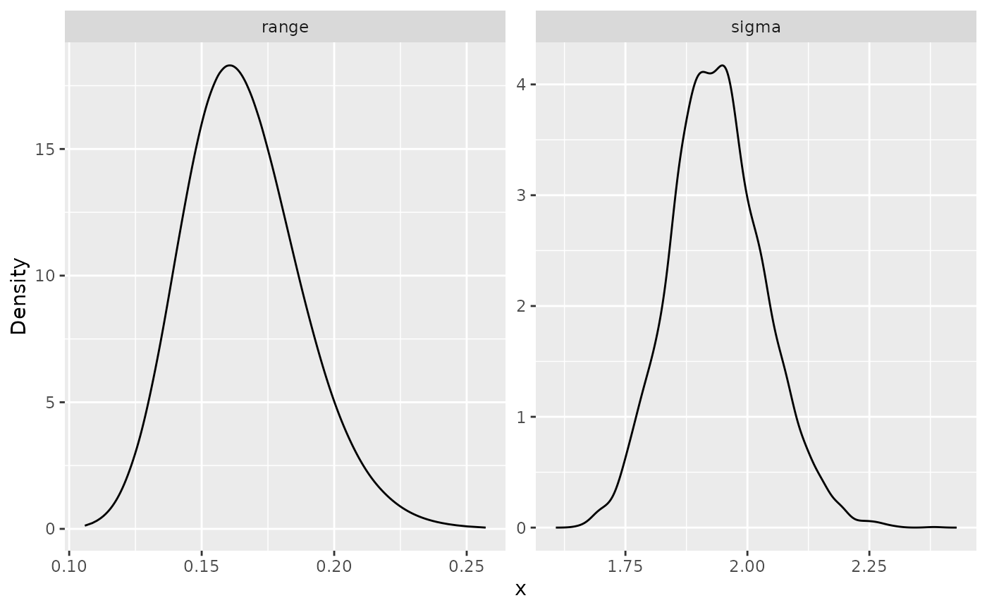

Kriging with the inlabru implementation

Unfortunately, our inlabru implementation is not compatible with inlabru’s predict() method. This has to do with the nature of the metric graph’s object.

To this end, we have provided a different predict() method. We will now show how to do kriging with the help of this function.

We begin by creating a data list with the positions we want the predictions. In this case, we will want the predictions on a mesh.

The positions we want are the mesh positions, which we have in the data.frame for the previous models. The function graph_bru_process_data() helps us into converting that data.frame to an inlabru friendly format for dealing with metric graphs:

data_list <- graph_bru_process_data(data_mesh_pred, loc = "loc")

We can now obtain the predictions by using the predict() method. Observe that our predict() method for graph models is a bit different from inlabru’s standard predict() method. Indeed, the first argument is the model created with the graph_spde() function, the second is inlabru’s component, and the remaining is as done with the standard predict() method in inlabru.

field_pred <- predict(spde_model, 
                                cmp,
                                spde_bru_fit, 
                                newdata = data_list,
                                formula = ~ field)

## Warning in (function (formula = . ~ ., family = "gaussian", data = NULL, : Non data-frame list-like data supplied; guessing allow_combine=TRUE.
##   Specify allow_combine explicitly to avoid this warning.

Let us plot the predictions of the latent field:

mean_field_prd <- field_pred$pred[,1]
graph$plot_function(X = mean_field_prd, 
                      vertex_size = 0, edge_width = 0.5,
                      type = "mapview")

Finally, let us plot predictions of the observed data at the mesh locations:

obs_pred <- predict(spde_model, 
                                cmp,
                                spde_bru_fit, 
                                newdata = data_list,
                                formula = ~ Intercept + lat + lon + field)

## Warning in (function (formula = . ~ ., family = "gaussian", data = NULL, : Non data-frame list-like data supplied; guessing allow_combine=TRUE.
##   Specify allow_combine explicitly to avoid this warning.

Let us plot the predictions:

mean_obs_prd <- obs_pred$pred[,1]
graph$plot_function(X = mean_obs_prd, 
                    vertex_size = 0, edge_width = 0.5,
                    type = "mapview")

References

Anderes, Ethan, Jesper Møller, and Jakob G. Rasmussen. 2020. “Isotropic Covariance Functions on Graphs and Their Edges.” Annals of Statistics 48: 2478–2503.

Bachl, Fabian E., Finn Lindgren, David L. Borchers, and Janine B. Illian. 2019. “Inlabru: An r Package for Bayesian Spatial Modelling from Ecological Survey Data.” Methods in Ecology and Evolution 10: 760–66.

Bivand, Roger S., Edzer Pebesma, and Virgilio Gomez-Rubio. 2013. Applied Spatial Data Analysis with r. Springer, NY.

Bolin, David, Alexandre B. Simas, and Jonas Wallin. 2023. “Statistical Properties of Gaussian Whittle–Matérn Fields on Metric Graphs.” arXiv:2304.10372.

———. 2024. “Gaussian Whittle–Matérn Fields on Metric Graphs.” Bernoulli 30: 1611–39.

Borovitskiy, Viacheslav, Iskander Azangulov, Alexander Terenin, Peter Mostowsky, Marc Deisenroth, and Nicolas Durrande. 2021. “Matérn Gaussian Processes on Graphs.” International Conference on Artificial Intelligence and Statistics, 2593–2601.

Lindgren, Finn, and Haavard Rue. 2015. “Bayesian Spatial Modelling with r-INLA.” Journal of Statistical Software 63: 1–25.

Sievert, Carson. 2020. Interactive Web-Based Data Visualization with r, Plotly, and Shiny. Chapman; Hall/CRC.