Working with metric graphs
David Bolin, Alexandre B. Simas, and Jonas Wallin
Created: 2022-11-23. Last modified: 2026-05-14.
Source:vignettes/metric_graph.Rmd
metric_graph.RmdIntroduction
Networks such as street or river networks are examples of metric graphs. A compact metric graph consists of a set of finitely many vertices and a finite set of edges connecting the vertices. Each edge is a curve of finite length that connects two vertices. These curves are parameterized by arc length and a location is a position on an edge, and can thus be represented as a touple where . Compared to regular graphs, where one typically defines functions on the vertices, we are for metric graphs interested in function that are defined on both the vertices and the edges.
In this vignette we will introduce the metric_graph
class of the MetricGraph package. This class provides a
user friendly representation of metric graphs, and we will show how to
use the class to construct and visualize metric graphs, add data to
them, and work with functions defined on the graphs.
For details about Gaussian processes and inference on metric graphs, we refer to the Vignettes
Constructing metric graphs
Basic constructions and properties
A metric graph can be constructed in two ways. The first is to
specify all edges in the graph as a list object, where each
entry is a matrix. To illustrate this, we first construct the following
edges
edge1 <- rbind(c(0,0),c(1,0))
edge2 <- rbind(c(0,0),c(0,1))
edge3 <- rbind(c(0,1),c(-1,1))
theta <- seq(from=pi,to=3*pi/2,length.out = 50)
edge4 <- cbind(sin(theta),1+ cos(theta))
edges = list(edge1, edge2, edge3, edge4)We can now create the graph based on the edges object as
follows
graph <- metric_graph$new(edges = edges)
graph$plot()
The plot function that was used to create the plot above has various
parameters to set the sizes and colors of the vertices and edges, and it
has a plotly argument to visualize the graph in 3D. For
this to work, the plotly library must be installed.
graph$plot(type = "plotly", vertex_size = 5, vertex_color = "blue",
edge_color = "red", edge_width = 2)It is also important to know that the 2d version of the
plot() method returns a ggplot2 object and can
be modified as such. For instance:
p <- graph$plot()
p + ggplot2::labs(title = "Metric graph",
x = "long", y = "lat")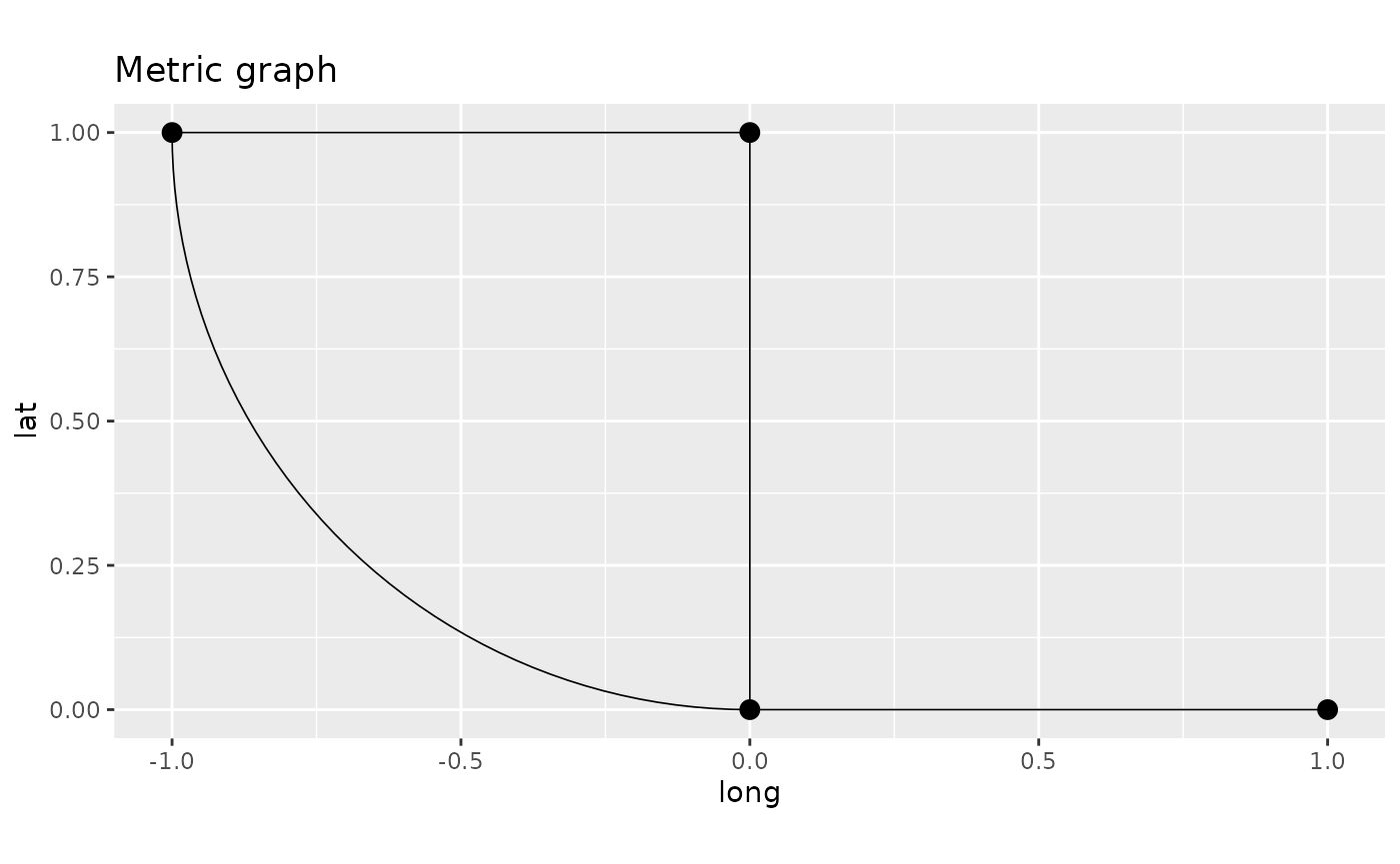
Similarly, the 3d version of the plot()
method returns a plotly object that can also be modified.
For instance:
p <- graph$plot(type = "plotly")
p <- plotly::layout(p, title = "Metric graph",
scene = list(xaxis=
list(title = "Long"),yaxis=list(title = "Lat")))
pWe can now obtain various properties of the graph: The vertex matrix, which specifies the Euclidian coordinates of the vertices is
graph$V## X Y
## [1,] 0 0
## [2,] 1 0
## [3,] 0 1
## [4,] -1 1and the edge matrix that specified the edges of the graph (i.e., which vertices that are connected by edges) is
graph$E## [,1] [,2]
## [1,] 1 2
## [2,] 1 3
## [3,] 3 4
## [4,] 1 4To obtain the geodesic (shortest path) distance between the vertices,
we can use the function compute_geodist:
graph$compute_geodist()
graph$geo_dist## $.vertices
## [,1] [,2] [,3] [,4]
## [1,] 0.000000 1.000000 1 1.570729
## [2,] 1.000000 0.000000 2 2.570729
## [3,] 1.000000 2.000000 0 1.000000
## [4,] 1.570729 2.570729 1 0.000000The second option it to construct the graph using two matrices
V and E that specify the locations (in
Euclidean space) of the vertices and the edges. In this case, it is
assumed that the graph only has straight edges:
V <- rbind(c(0, 0), c(1, 0), c(0, 1), c(-1, 1))
E <- rbind(c(1, 2), c(1, 3), c(3, 4), c(4, 1))
graph2 <- metric_graph$new(V = V, E = E)## Starting graph creation...## LongLat is set to FALSE## Creating edges...## Setting edge weights...## Computing bounding box...## Setting up edges## Merging close vertices## Total construction time: 0.27 secs## Creating and updating vertices...## Storing the initial graph...## Computing the relative positions of the edges...
graph2$plot()
A third option is to create a graph from a SpatialLines
object:
library(sp)
line1 <- Line(rbind(c(0,0),c(1,0)))
line2 <- Line(rbind(c(0,0),c(0,1)))
line3 <- Line(rbind(c(0,1),c(-1,1)))
theta <- seq(from=pi,to=3*pi/2,length.out = 50)
line4 <- Line(cbind(sin(theta),1+ cos(theta)))
Lines = sp::SpatialLines(list(Lines(list(line1),ID="1"),
Lines(list(line2),ID="2"),
Lines(list(line3),ID="3"),
Lines(list(line4),ID="4")))
graph <- metric_graph$new(edges = Lines)
graph$plot()
A final option is to create from a MULTILINESTRING
object:
library(sf)
line1 <- st_linestring(rbind(c(0,0),c(1,0)))
line2 <- st_linestring(rbind(c(0,0),c(0,1)))
line3 <- st_linestring(rbind(c(0,1),c(-1,1)))
theta <- seq(from=pi,to=3*pi/2,length.out = 50)
line4 <- st_linestring(cbind(sin(theta),1+ cos(theta)))
multilinestring = st_multilinestring(list(line1, line2, line3, line4))
graph <- metric_graph$new(edges = multilinestring)
graph$plot()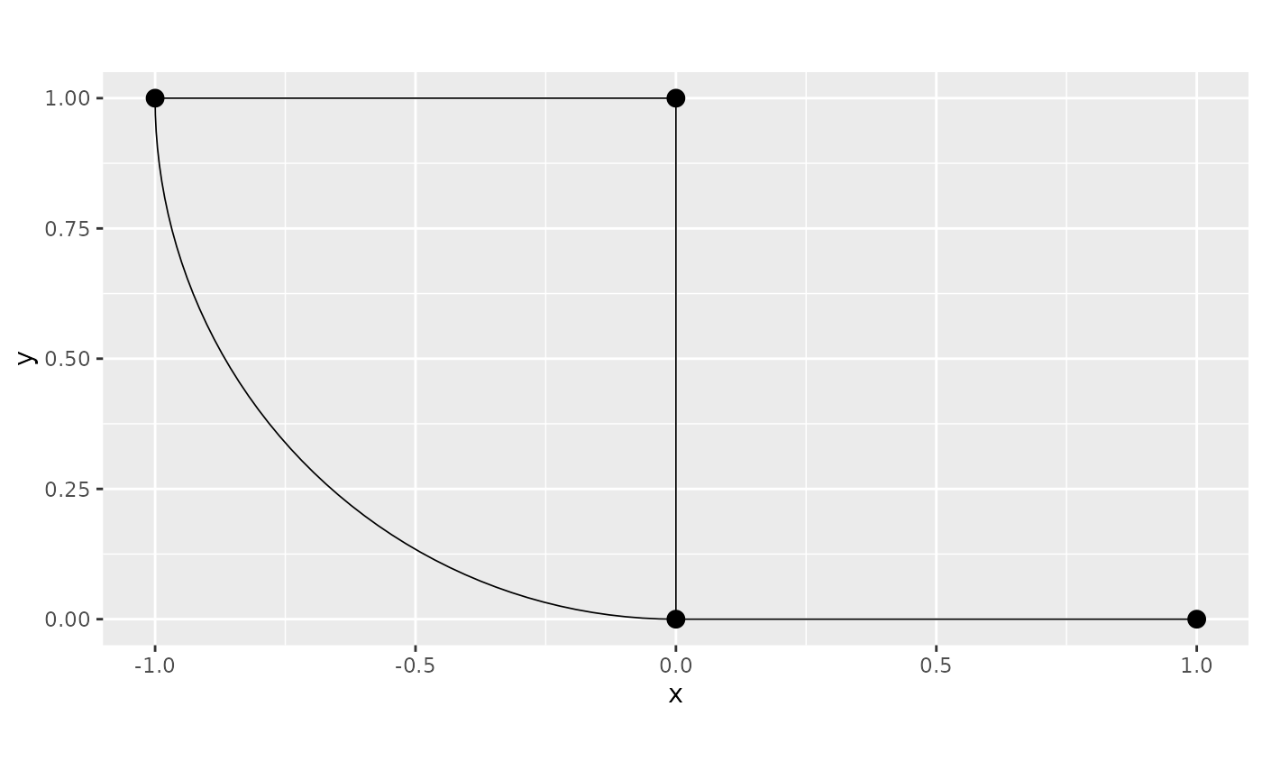
Tolerances for merging vertices and edges
The constructor of the graph has one argument,
perform_merges and an additional argument
tolerance which is used for connecting edges that are close
in Euclidean space. Specifically, the tolerance argument is
given as a list with three elements:
-
vertex_vertexvertices that are closer than this number are merged (the default value is1e-7) -
vertex_edgeif a vertex at the end of one edge is closer than this number to another edge, this vertex is connected to that edge (the default value is1e-7) -
edge_edgeif two edges at some point are closer than this number, a new vertex is added at that point and the two edges are connected (the default value is0which means that the option is not used)
These options are often needed when constructing graphs based on real
data, for example from OpenStreetMap as we will see later. To illustrate
these options, suppose that we want to construct a graph from the
following three edges. We will set perform_merges to
TRUE, to show how they are merged with the default choice
of tolerances.
edge1 <- rbind(c(0,0),c(1,0))
edge2 <- rbind(c(0,0.03),c(0,0.75))
edge3 <- rbind(c(-1,1),c(0.5,0.03))
edge4 <- rbind(c(0,0.75), c(0,1))
edge5 <- rbind(c(-1,0), c(-1, 0.9995))
edges = list(edge1, edge2, edge3, edge4, edge5)
graph3 <- metric_graph$new(edges = edges, perform_merges = TRUE)
graph3$plot(degree = TRUE)
print(graph3$nV)## [1] 8
We added the option degree=TRUE to the plot here to
visualize the degrees of each vertex. As expected, one sees that all
vertices have degree 1, and none of the three edges are connected. If
these are streets in a street network, one might suspect that the two
vertices at
and
really should be the same vertex so that the two edges are connected.
This can be adjusted by increasing the vertex_vertex
tolerance:
graph3 <- metric_graph$new(edges = edges, perform_merges = TRUE,
tolerance = list(vertex_vertex = 0.05))
graph3$plot(degree = TRUE)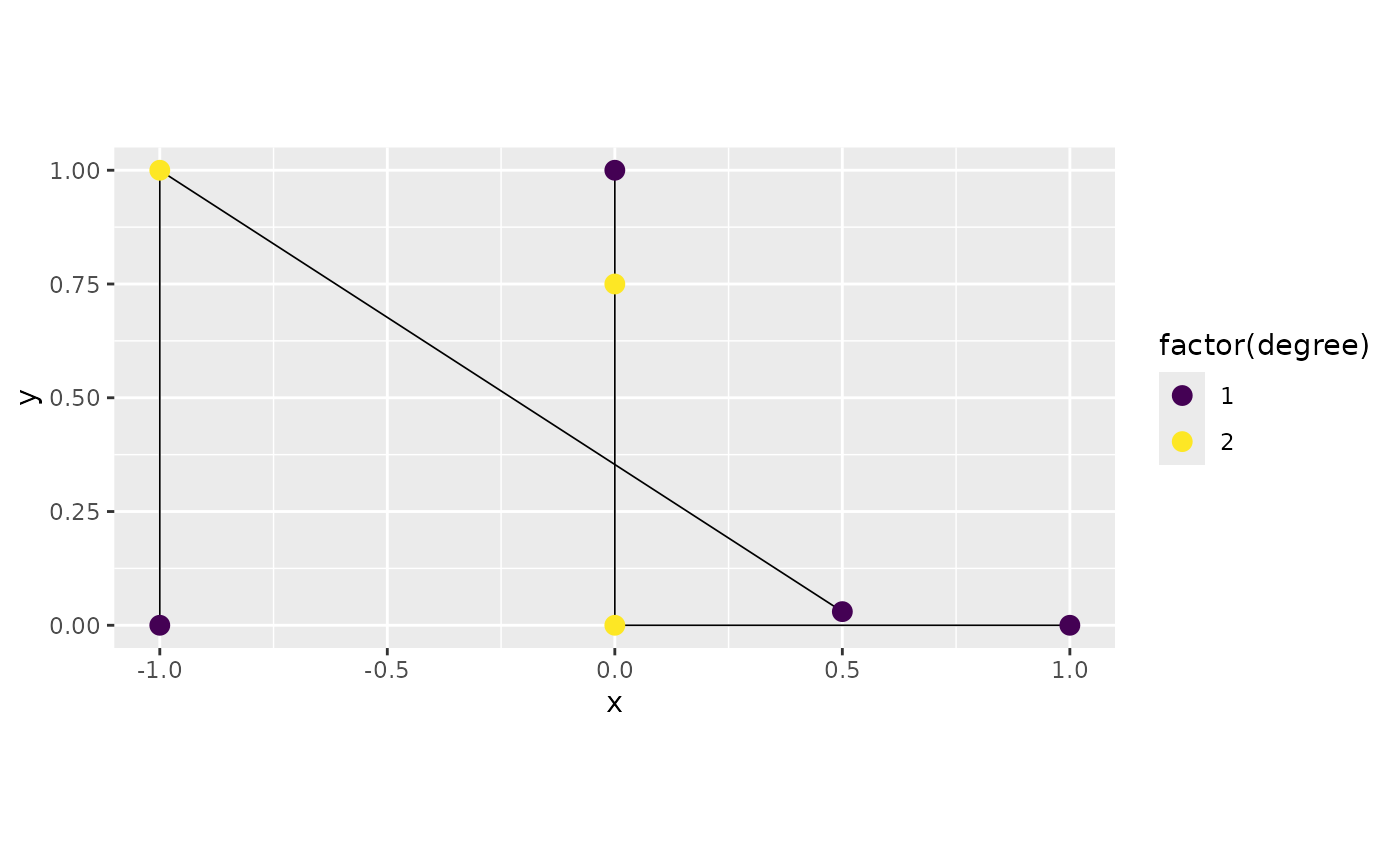
One might also want to add the vertex at
as a vertex on the first edge, so that the two edges there are
connected. This can be done by adjusting the vertex_edge
tolerance:
graph3 <- metric_graph$new(edges = edges, perform_merges = TRUE,
tolerance = list(vertex_vertex = 0.05,
vertex_edge = 0.1))
graph3$plot(degree = TRUE)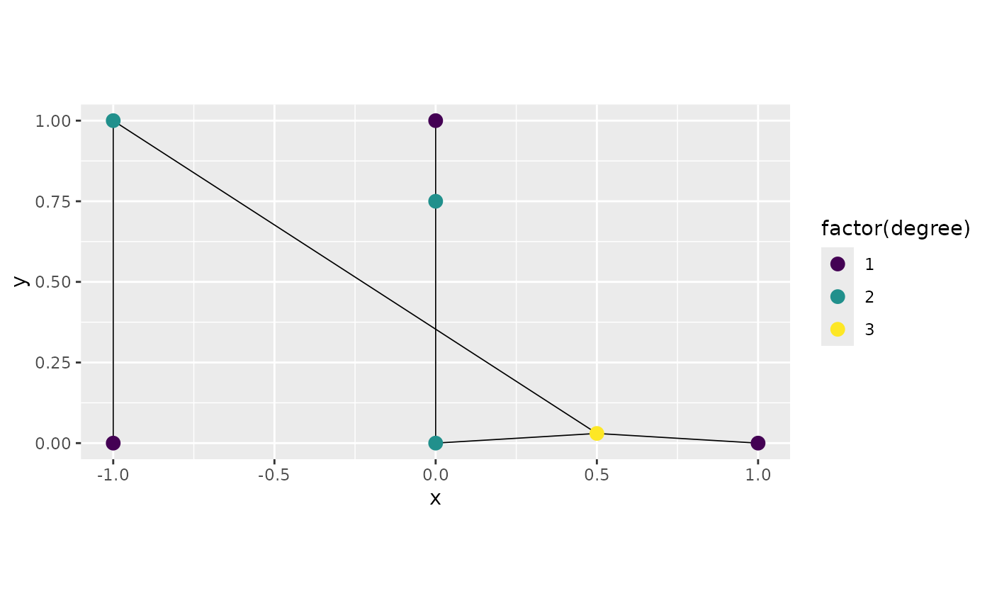
We can see that the vertex at
was indeed connected with the edge from
to
and that vertex now has degree 3 since it is connected with three edges.
One can also note that the edges object that was used to
create the graph is modified internally in the metric_graph
object so that the connections are visualized correctly in the sense
that all edges are actually shown as connected edges.
Finally, to add a vertex at the intersection between
edge2 and edge3 we can adjust the
edge_edge tolerance:
graph3 <- metric_graph$new(edges = edges, perform_merges = TRUE,
tolerance = list(vertex_vertex = 0.2,
vertex_edge = 0.1,
edge_edge = 0.001))
graph3$plot(degree = TRUE)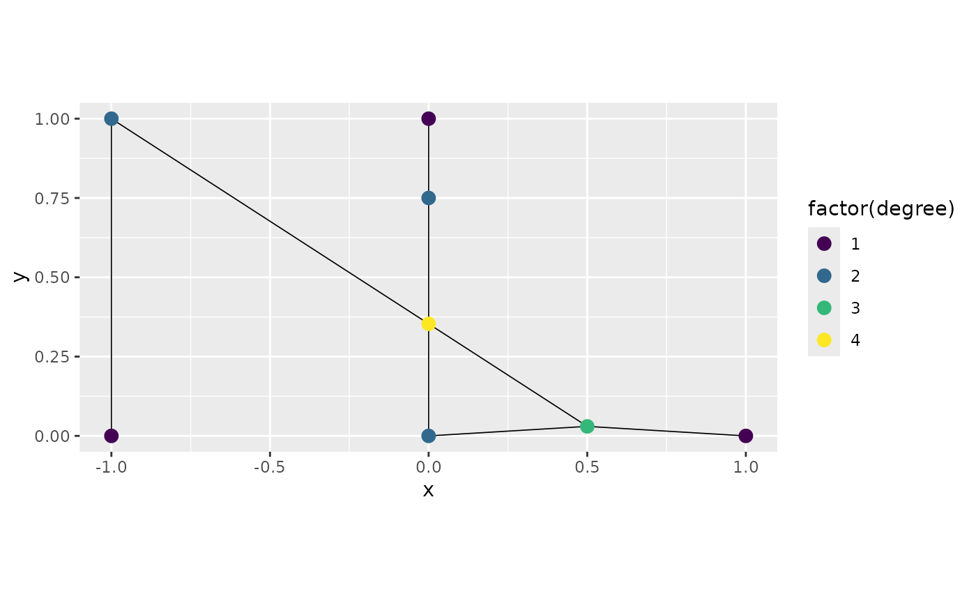
Now, the structure of the metric graph does not change if we add or
remove vertices of degree 2. Because of this,one might want to remove
vertices of degree 2 since this can reduce computational costs. This can
be done by setting the remove_deg2 argument while creating
the graph:
graph3 <- metric_graph$new(edges = edges, perform_merges = TRUE,
tolerance = list(vertex_vertex = 0.2,
vertex_edge = 0.1,
edge_edge = 0.001),
remove_deg2 = TRUE)
graph3$plot(degree = TRUE)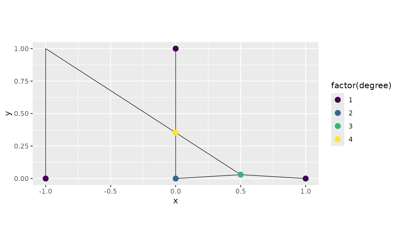
Observe that one vertex of degree 2 was not removed. This is due to
the fact that if we consider the direction, this vertex has directions
incompatible for removal. We can see this by setting the argument
direction=TRUE in the plot() method:
graph3$plot(direction = TRUE)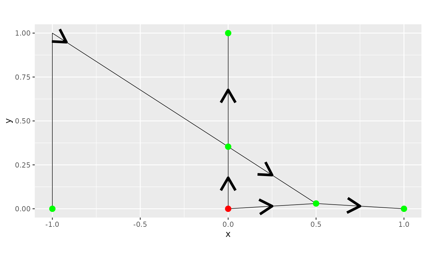
We can also avoid performing these merges by setting using the
default constructor (which is equivalent to set the
perform_merges argument to FALSE):
graph4 <- metric_graph$new(edges = edges)
graph4$plot(degree = TRUE)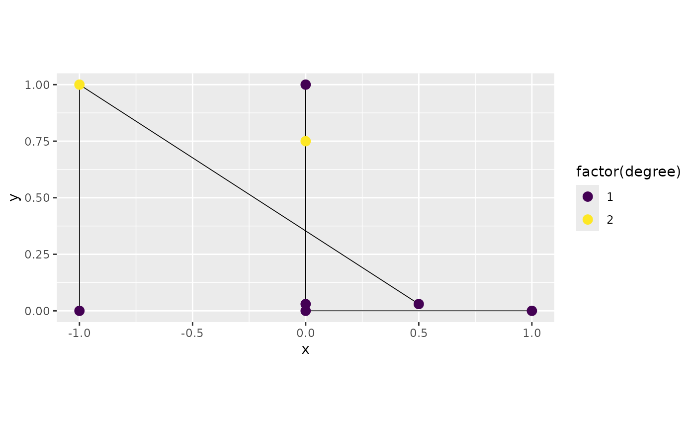
Observe that the two vertices around the point
were merged. This is because there is an additional step to merge close
vertices that is performed even with perform_merges set to
FALSE. To also skip this merge, we can also set
merge_close_vertices to FALSE:
graph4 <- metric_graph$new(edges = edges, merge_close_vertices=FALSE)
graph4$plot(degree = TRUE)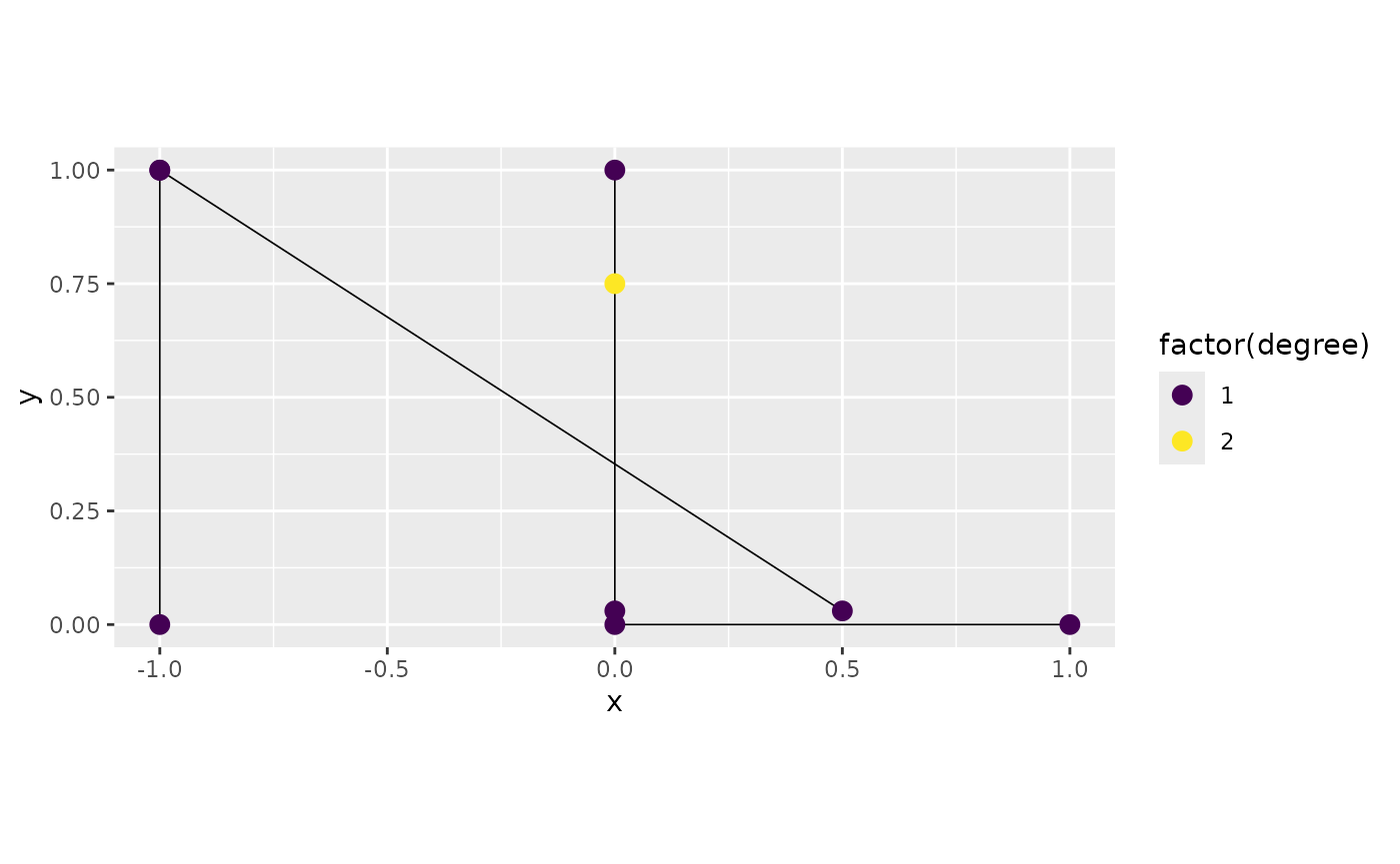
We can see now that the two vertices around the point were not merged.
Edge lengths
Whenever we create a metric graph, the edge lengths will be automatically computed by obtaining the lengths of the edges. However, sometimes one might want to provide manual edge lengths.
Let us consider the following example:
library(sp)
line1 <- Line(rbind(c(0,0),c(1,0)))
line2 <- Line(rbind(c(0,0),c(0,1)))
line3 <- Line(rbind(c(0,1),c(-1,1)))
theta <- seq(from=pi,to=3*pi/2,length.out = 25)
line4 <- Line(cbind(sin(theta),1+ cos(theta)))
Lines = sp::SpatialLines(list(Lines(list(line1),ID="1"),
Lines(list(line2),ID="2"),
Lines(list(line3),ID="3"),
Lines(list(line4),ID="4")))
graph <- metric_graph$new(edges = Lines)
graph$plot()
We can obtain the edge lenghts by using the
get_edge_lengths() method:
graph$get_edge_lengths()## [1] 1.000000 1.000000 1.000000 1.570516Observer that we know that the actual length of edge 4 is , which is not quite right (observe that edge 4 is an approximation of a quarter of a circle by a polygon with 25 points):
pi/2 - graph$get_edge_lengths()[4]## [1] 0.0002803513We can provide the actual edge lengths, by using the
set_manual_edge_lengths() method:
graph$set_manual_edge_lengths(c(1,1,1,pi/2))
graph$get_edge_lengths()## [1] 1.000000 1.000000 1.000000 1.570796We can also manually provide the edge lengths when creating the metric graph:
graph <- metric_graph$new(edges = Lines, manual_edge_lengths = c(1,1,1,pi/2))
graph$get_edge_lengths() ## [1] 1.000000 1.000000 1.000000 1.570796However, it is important to note that if one passes the
manual_edge_lengths when creating the graph, it will automatically set
perform_merges to FALSE, as there is no
consistent way to obtain the edge lengths after the merges from the
manual edge lengths. Nevertheless, merge_close_vertices can
be set to TRUE.
Characteristics of the graph
A brief summary of the main characteristics of the graph can be
obtained by the compute_characteristics() method:
graph3$compute_characteristics()We can, then, view those characteristics by simply printing the
metric_graph object:
graph3## A metric graph with 6 vertices and 6 edges.
##
## Vertices:
## Degree 1: 3; Degree 2: 1; Degree 3: 1; Degree 4: 1;
## With incompatible directions: 1
##
## Edges:
## Lengths:
## Min: 0.3533333 ; Max: 2.190873 ; Total: 4.788107
## Weights:
## Min: 1 ; Max: 1
## That are circles: 0
##
## Graph units:
## Vertices unit: None ; Lengths unit: None
##
## Longitude and Latitude coordinates: FALSE
##
## Some characteristics of the graph:
## Connected: TRUE
## Has loops: FALSE
## Has multiple edges: FALSE
## Is a tree: FALSE
## Distance consistent: unknown## To check if the graph satisfies the distance consistency, run the `check_distance_consistency()` method.## Has Euclidean edges: unknown## To check if the graph has Euclidean edges, run the `check_euclidean()` method.Observe that we do not know that the graph has Euclidean edges. We
can check by using the check_euclidean() method:
graph3$check_euclidean()Let us view the characteristics again:
graph3## A metric graph with 6 vertices and 6 edges.
##
## Vertices:
## Degree 1: 3; Degree 2: 1; Degree 3: 1; Degree 4: 1;
## With incompatible directions: 1
##
## Edges:
## Lengths:
## Min: 0.3533333 ; Max: 2.190873 ; Total: 4.788107
## Weights:
## Min: 1 ; Max: 1
## That are circles: 0
##
## Graph units:
## Vertices unit: None ; Lengths unit: None
##
## Longitude and Latitude coordinates: FALSE
##
## Some characteristics of the graph:
## Connected: TRUE
## Has loops: FALSE
## Has multiple edges: FALSE
## Is a tree: FALSE
## Distance consistent: TRUE
## Has Euclidean edges: TRUEIt can happen that we have that the graph does not have Euclidean
edges without the need to check the distance consistency. However, if
one wants to check if the graph satisfies the distance consistency
assumption, one can run the check_distance_consistency()
function:
graph3$check_distance_consistency()Further, the individual characteristics can be accessed (after
running the compute_characteristics() method) through the
characteristics component of the graph object:
graph3$characteristics## $has_loops
## [1] FALSE
##
## $connected
## [1] TRUE
##
## $has_multiple_edges
## [1] FALSE
##
## $is_tree
## [1] FALSE
##
## $distance_consistency
## [1] TRUE
##
## $euclidean
## [1] TRUESummaries of metric graphs
We can also obtain a summary of the informations contained on a
metric graph object by using the summary() method. Let us
obtain a summary of informations of graph3:
summary(graph3)## A metric graph object with:
##
## Vertices:
## Total: 6
## Degree 1: 3; Degree 2: 1; Degree 3: 1; Degree 4: 1;
## With incompatible directions: 1
##
## Edges:
## Total: 6
## Lengths:
## Min: 0.3533333 ; Max: 2.190873 ; Total: 4.788107
## Weights:
## Min: 1 ; Max: 1
## That are circles: 0
##
## Graph units:
## Vertices unit: None ; Lengths unit: None
##
## Longitude and Latitude coordinates: FALSE
##
## Some characteristics of the graph:
## Connected: TRUE
## Has loops: FALSE
## Has multiple edges: FALSE
## Is a tree: FALSE
## Distance consistent: TRUE
## Has Euclidean edges: TRUE
##
## Computed quantities inside the graph:
## Laplacian: FALSE ; Geodesic distances: TRUE
## Resistance distances: FALSE ; Finite element matrices: FALSE
##
## Mesh: The graph has no mesh!
##
## Data: The graph has no data!
##
## Tolerances:
## vertex-vertex: 0.2
## vertex-edge: 0.1
## edge-edge: 0.001Observe that there are some quantities that were not computed on the
summary. We can see how to compute them by setting the argument
messages to TRUE:
summary(graph3, messages = TRUE)## A metric graph object with:
##
## Vertices:
## Total: 6
## Degree 1: 3; Degree 2: 1; Degree 3: 1; Degree 4: 1;
## With incompatible directions: 1
##
## Edges:
## Total: 6
## Lengths:
## Min: 0.3533333 ; Max: 2.190873 ; Total: 4.788107
## Weights:
## Min: 1 ; Max: 1
## That are circles: 0
##
## Graph units:
## Vertices unit: None ; Lengths unit: None
##
## Longitude and Latitude coordinates: FALSE
##
## Some characteristics of the graph:
## Connected: TRUE
## Has loops: FALSE
## Has multiple edges: FALSE
## Is a tree: FALSE
## Distance consistent: TRUE
## Has Euclidean edges: TRUE
##
## Computed quantities inside the graph:
## Laplacian: FALSE ; Geodesic distances: TRUE## To compute the Laplacian, run the 'compute_laplacian()' method.## Resistance distances: FALSE ; Finite element matrices: FALSE## To compute the resistance distances, run the 'compute_resdist()' method.## To compute the finite element matrices, run the 'compute_fem()' method.##
## Mesh: The graph has no mesh!## To build the mesh, run the 'build_mesh()' method.##
## Data: The graph has no data!## To add observations, use the 'add_observations()' method.##
## Tolerances:
## vertex-vertex: 0.2
## vertex-edge: 0.1
## edge-edge: 0.001Finally, the summary() can also be accessed from the
metric graph object:
graph3$summary()## A metric graph object with:
##
## Vertices:
## Total: 6
## Degree 1: 3; Degree 2: 1; Degree 3: 1; Degree 4: 1;
## With incompatible directions: 1
##
## Edges:
## Total: 6
## Lengths:
## Min: 0.3533333 ; Max: 2.190873 ; Total: 4.788107
## Weights:
## Min: 1 ; Max: 1
## That are circles: 0
##
## Graph units:
## Vertices unit: None ; Lengths unit: None
##
## Longitude and Latitude coordinates: FALSE
##
## Some characteristics of the graph:
## Connected: TRUE
## Has loops: FALSE
## Has multiple edges: FALSE
## Is a tree: FALSE
## Distance consistent: TRUE
## Has Euclidean edges: TRUE
##
## Computed quantities inside the graph:
## Laplacian: FALSE ; Geodesic distances: TRUE
## Resistance distances: FALSE ; Finite element matrices: FALSE
##
## Mesh: The graph has no mesh!
##
## Data: The graph has no data!
##
## Tolerances:
## vertex-vertex: 0.2
## vertex-edge: 0.1
## edge-edge: 0.001Vertices and edges
The metric graph object has the edges and
vertices elements in its list. We can get a quick summary
from them by calling these elements:
graph3$vertices## Vertices of the metric graph
##
## Longitude and Latitude coordinates: FALSE
##
## Summary:
## x y Degree Indegree Outdegree Problematic
## 1 0.0 0.0000000 2 0 2 TRUE
## 2 1.0 0.0000000 1 1 0 FALSE
## 3 0.5 0.0300000 3 2 1 FALSE
## 4 0.0 1.0000000 1 0 1 FALSE
## 5 -1.0 0.0000000 1 1 0 FALSE
## 6 0.0 0.3533333 4 2 2 FALSEand
graph3$edges## Edges of the metric graph
##
## Longitude and Latitude coordinates: FALSE
##
## Summary:
##
## Edge 1 (first and last coordinates):
## x y
## 0.0 0.00
## 0.5 0.03
## Total number of coordinates: 2
## Edge length: 0.5008992
## Weight: 1
##
## Kirchhoff weight: 1
##
## Directional weight: 1
##
## Edge 2 (first and last coordinates):
## x y
## 0 0.0000000
## 0 0.3533333
## Total number of coordinates: 2
## Edge length: 0.3533333
## Weight: 1
##
## Kirchhoff weight: 1
##
## Directional weight: 1
##
## Edge 3 (first and last coordinates):
## x y
## 0 0.3533333
## -1 0.0000000
## Total number of coordinates: 3
## Edge length: 2.190873
## Weight: 1
##
## Kirchhoff weight: 1
##
## Directional weight: 1
##
## Edge 4 (first and last coordinates):
## x y
## 0 1.0000000
## 0 0.3533333
## Total number of coordinates: 3
## Edge length: 0.6466667
## Weight: 1
##
## Kirchhoff weight: 1
##
## Directional weight: 1## # 2 more edges## # Use `print(n=...)` to see more edgesWe can also look at individual edges and vertices. For example, let us look at vertice number 2:
graph3$vertices[[2]]## Vertex 2 of the metric graph
##
## Longitude and Latitude coordinates: FALSE
##
## Summary:
## x y Degree Indegree Outdegree Problematic
## 1 0 1 1 0 FALSESimilarly, let us look at edge number 4:
graph3$edges[[4]]## Edge 4 of the metric graph
##
## Longitude and Latitude coordinates: FALSE
##
## Coordinates of the vertices of the edge:
## x y
## 0 1.0000000
## 0 0.3533333
##
## Coordinates of the edge:
## x y
## 0 1.0000000
## 0 0.7500000
## 0 0.3533333
##
## Relative positions of the edge:
## Edge number Distance on edge
## 4 0.0000000
## 4 0.3865979
## 4 1.0000000
##
## Total number of coordinates: 3
## Edge length: 0.6466667
## Weight: 1
## Kirchhoff weight: 1
##
## Directional weight: 1We have a message informing us that the relative positions of the
edges were not computed. They are used to produce better plots when
using the plot_function() method, see the section
“Improving the plot obtained by plot_function” below. To
compute the relative positions, we run the
compute_PtE_edges() method:
graph3$compute_PtE_edges()Now, we take a look at edge number 4 again:
graph3$edges[[4]]## Edge 4 of the metric graph
##
## Longitude and Latitude coordinates: FALSE
##
## Coordinates of the vertices of the edge:
## x y
## 0 1.0000000
## 0 0.3533333
##
## Coordinates of the edge:
## x y
## 0 1.0000000
## 0 0.7500000
## 0 0.3533333
##
## Relative positions of the edge:
## Edge number Distance on edge
## 4 0.0000000
## 4 0.3865979
## 4 1.0000000
##
## Total number of coordinates: 3
## Edge length: 0.6466667
## Weight: 1
## Kirchhoff weight: 1
##
## Directional weight: 1Understanding coordinates on graphs
The locations of the vertices are specified in Euclidean coordinates.
However, when specifying a position on the graph, it is not practical to
work with Euclidean coordinates since not all locations in Euclidean
space are locations on the graph. It is instead better to specify a
location on the graph by the touple
,
where
denotes the number of the edge and
is the location on the edge. The location
can either be specified as the distance from the start of the edge (and
then takes values between 0 and the length of the edge) or as the
normalized distance from the start of the edge (and then takes values
between 0 and 1). The function coordinates can be used to
convert between coordinates in Euclidean space and locations on the
graph. For example the location at distance 0.2 from the start of the
second edge is:
## [,1] [,2]
## [1,] 0 0.2In this case, since the edge has length 1, the location of the point at normalized distance 0.2 from the start of the edge is the same:
## [,1] [,2]
## [1,] 0 0.2The function can also be used to find the closest location on the graph for a location in Euclidean space:
## [,1] [,2]
## [1,] 2 0.2In this case, the normalized argument decides whether
the returned value should be given in normalized distance or not.
Methods for working with real data
To illustrate the useage of metric_graph on some real
data, we use the osmdata package to download data from
OpenStreetMap. In the following code, we extract highways for a part of
the city of Copenhagen:
library(osmdata)
bbox <- c(12.5900, 55.6000, 12.6850, 55.6450)
call <- opq(bbox)
call <- add_osm_feature(call, key = "highway",value=c("motorway", "primary",
"secondary", "tertiary"))
data_sf <- osmdata_sf(call)
graph5 <- metric_graph$new(lapply(data_sf$osm_lines$geometry,
function(dat){sf::st_coordinates(dat)[,1:2]}))
graph5$plot(vertex_size = 0)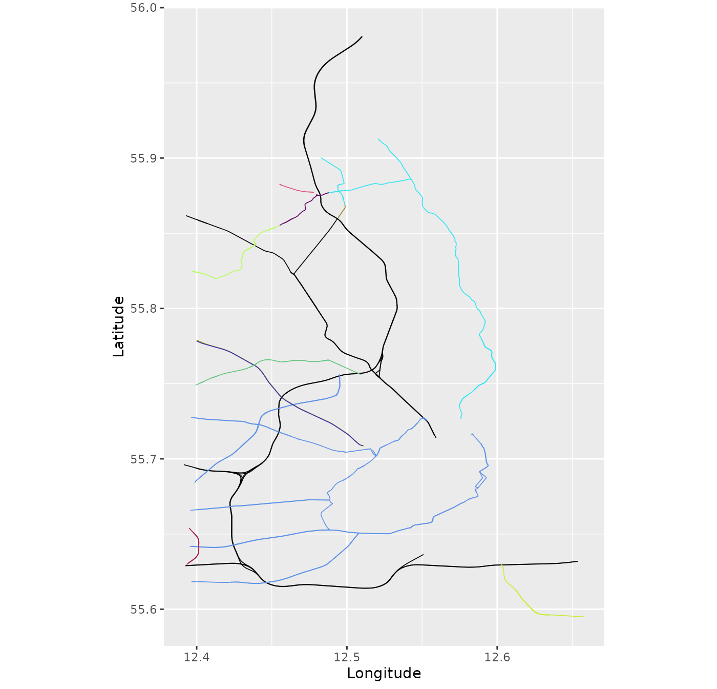
There are a few things to note about data like this. The first is that the coordinates are given in Longitude and Latitude. Because of this, the edge lengths are by default given in degrees, which may result in very small numbers:
range(graph5$get_edge_lengths())## [1] 6.516993e-05 5.636913e-02This may cause numerical instabilities when dealing with random
fields on the graph, and it also makes it difficult to interpret results
(unless one has a good intuition about distances in degrees). To avoid
such problems, it is better to set the longlat argument
when constructing the graph:
graph5 <- metric_graph$new(lapply(data_sf$osm_lines$geometry,
function(dat){sf::st_coordinates(dat)[,1:2]}), longlat = TRUE)This tells the constructor that the coordinates are given in Longitude and Latitude and that distances should be calculated in km. So if we now look at the edge lengths, they are given in km:
range(graph5$get_edge_lengths())## Units: [km]
## [1] 0.001650041 4.042991481Alternatively, and more conveniently, whenever the sf
object has a valid crs, it will automatically use this
crs to set the correct coordinate reference system (CRS) in
the metric graph. Above, we ended up removing the crs when
we created the linestring object from the resulting
osm_lines. Let us, instead, build the graph directly using
the osmdata_sf object:
graph5 <- metric_graph$new(data_sf)We can see now that graph5 automatically has the correct
CRS:
graph5## A metric graph with 347 vertices and 366 edges.
##
## Vertices:
## Degree 1: 29; Degree 2: 266; Degree 3: 39; Degree 4: 11; Degree 5: 2;
## With incompatible directions: 5
##
## Edges:
## Lengths:
## Min: 0.001650041 ; Max: 4.042991 ; Total: 68.82467
## Weights:
## Columns: osm_id name alt_name animal_crossing:animal bicycle bridge cycleway cycleway:both cycleway:left cycleway:right cycleway:width destination destination:lanes destination:ref destination:symbol foot hazard hazmat:conditional highway horse int_ref junction lane_markings lanes lanes:backward lanes:forward layer lit mapillary maxheight maxspeed maxspeed:advisory maxspeed:variable maxweight:signed mofa motorcar name:etymology name:etymology:wikidata name:etymology:wikipedia name:sv noname note oneway operator operator:wikidata operator:wikipedia placement priority ref shoulder sidewalk sidewalk:both:surface sidewalk:left sidewalk:left:surface sidewalk:right sidewalk:right:surface smoothness source:maxspeed start_date surface toll traffic_calming tunnel tunnel:alt_name:da tunnel:alt_name:sv tunnel:name tunnel:name:da tunnel:name:de tunnel:name:en tunnel:name:sv tunnel:official_name turn:lanes turn:lanes:backward turn:lanes:forward width wikidata .weights
## That are circles: 0
##
## Graph units:
## Vertices unit: degree ; Lengths unit: km
##
## Longitude and Latitude coordinates: TRUE
## Which spatial package: sp
## CRS: EPSG:4326This also allows us to plot the graph interactively with the
underlying world map, if the data has a coordinate reference system, by
setting type = "mapview" in the plot()
method:
graph5$plot(type = "mapview", vertex_size = 0)We can also check the edge lengths:
range(graph5$get_edge_lengths())## Units: [km]
## [1] 0.001650041 4.042991481Another advantage of adding the osmdata object, is that
the metric graph automatically adds the edge observations as
edge_weights:
graph5$get_edge_weights()## # A tibble: 366 × 77
## osm_id name alt_name animal_crossing:anim…¹ bicycle bridge cycleway
## <chr> <chr> <chr> <chr> <chr> <chr> <chr>
## 1 1525051 Backersvej NA NA NA NA lane
## 2 1692808 Saltværksvej NA NA yes NA track
## 3 1698015 NA NA NA no NA NA
## 4 1700205 Tårnbyvej NA NA yes NA track
## 5 1754353 Løjtegårdsvej NA NA NA NA track
## 6 1880381 Stenlandsvej NA NA use_si… NA separate
## 7 1880526 A.P. Møllers… NA NA NA NA no
## 8 2373286 Kastruplundg… NA NA NA NA no
## 9 3431744 Kirstinehøj NA NA NA NA track
## 10 3431748 Tømmerupvej NA NA NA NA track
## # ℹ 356 more rows
## # ℹ abbreviated name: ¹`animal_crossing:animal`
## # ℹ 70 more variables: `cycleway:both` <chr>, `cycleway:left` <chr>,
## # `cycleway:right` <chr>, `cycleway:width` <chr>, destination <chr>,
## # `destination:lanes` <chr>, `destination:ref` <chr>,
## # `destination:symbol` <chr>, foot <chr>, hazard <chr>,
## # `hazmat:conditional` <chr>, highway <chr>, horse <chr>, int_ref <chr>, …We can also let the color of the edges be determined by some edge
weight. For example, let us take maxspeed:
graph5$plot(vertex_size = 0, edge_weight = "maxspeed",
type="mapview")## Warning in RColorBrewer::brewer.pal(n = length(levels(edges_sf[[edge_weight]])), : minimal value for n is 3, returning requested palette with 3 different levels## Warning: Found less unique colors (3) than unique zcol values (6)!
## Recycling color vector.
## Warning: Found less unique colors (3) than unique zcol values (6)!
## Recycling color vector.Similarly, we can also set the edge width based on an edge weight
(for this case, we can only use type = "ggplot", which is
the default). In this example we will choose the column
lanes to determine the edge widths. If the number of lanes
is not available, the edge will be removed (we will replace the
NAs by zero).
graph5$set_edge_weights(weights = graph5$mutate_weights(lanes = ifelse(is.na(lanes),0,lanes), lanes = as.numeric(lanes)))
graph5$plot(vertex_size = 0, edge_weight = "maxspeed", edge_width_weight = "lanes")
However, observe that the edge widths are always relative, with the
largest being set to edge_width. So, let us set
edge_width to 4 to make it easier to perceive the
differences:
graph5$set_edge_weights(weights = graph5$mutate_weights(lanes = ifelse(is.na(lanes),0,lanes), lanes = as.numeric(lanes)))
graph5$plot(vertex_size = 0, edge_weight = "maxspeed", edge_width_weight = "lanes", edge_width = 4)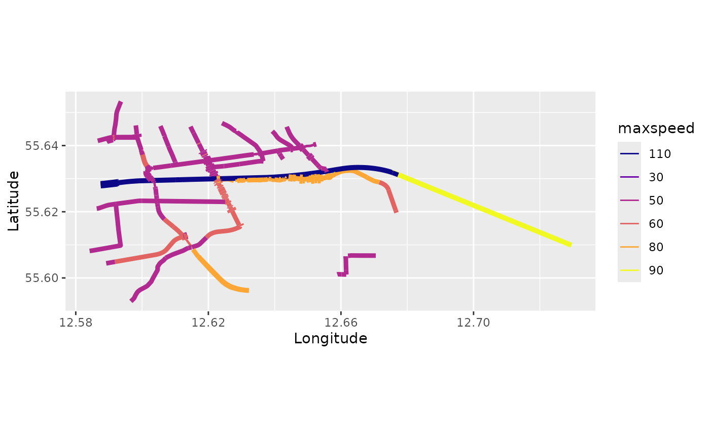
If one does not want to have the edge weights added, one must set
include_edge_weights to FALSE:
graph5 <- metric_graph$new(data_sf, include_edge_weights=FALSE)
graph5$get_edge_weights()## # A tibble: 366 × 1
## .weights
## <dbl>
## 1 1
## 2 1
## 3 1
## 4 1
## 5 1
## 6 1
## 7 1
## 8 1
## 9 1
## 10 1
## # ℹ 356 more rowsSimilarly, if one wants just to add some columns of the
osmdata object as edge weights, one can pass a vector with
the column names as the include_edge_weights argument. For
example, let us only get the columns highway and
lanes:
graph5 <- metric_graph$new(data_sf, include_edge_weights=c("highway", "lanes"))
graph5$get_edge_weights()## # A tibble: 366 × 3
## highway lanes .weights
## <chr> <chr> <dbl>
## 1 tertiary NA 1
## 2 tertiary 4 1
## 3 tertiary 1 1
## 4 tertiary 3 1
## 5 tertiary 1 1
## 6 tertiary 2 1
## 7 tertiary 2 1
## 8 tertiary 2 1
## 9 tertiary 3 1
## 10 tertiary 2 1
## # ℹ 356 more rowsThe same idea also works is one has an sf object
instead. Let us obtain the sf version from the
osmdata object:
data_sf <- osmdata_sf(call)We can now directly create the metric graph object:
graph5 <- metric_graph$new(data_sf)Let us check that graph5 still has the correct CRS:
graph5## A metric graph with 347 vertices and 366 edges.
##
## Vertices:
## Degree 1: 29; Degree 2: 266; Degree 3: 39; Degree 4: 11; Degree 5: 2;
## With incompatible directions: 5
##
## Edges:
## Lengths:
## Min: 0.001650041 ; Max: 4.042991 ; Total: 68.82467
## Weights:
## Columns: osm_id name alt_name animal_crossing:animal bicycle bridge cycleway cycleway:both cycleway:left cycleway:right cycleway:width destination destination:lanes destination:ref destination:symbol foot hazard hazmat:conditional highway horse int_ref junction lane_markings lanes lanes:backward lanes:forward layer lit mapillary maxheight maxspeed maxspeed:advisory maxspeed:variable maxweight:signed mofa motorcar name:etymology name:etymology:wikidata name:etymology:wikipedia name:sv noname note oneway operator operator:wikidata operator:wikipedia placement priority ref shoulder sidewalk sidewalk:both:surface sidewalk:left sidewalk:left:surface sidewalk:right sidewalk:right:surface smoothness source:maxspeed start_date surface toll traffic_calming tunnel tunnel:alt_name:da tunnel:alt_name:sv tunnel:name tunnel:name:da tunnel:name:de tunnel:name:en tunnel:name:sv tunnel:official_name turn:lanes turn:lanes:backward turn:lanes:forward width wikidata .weights
## That are circles: 0
##
## Graph units:
## Vertices unit: degree ; Lengths unit: km
##
## Longitude and Latitude coordinates: TRUE
## Which spatial package: sp
## CRS: EPSG:4326and the correct edge lengths:
range(graph5$get_edge_lengths())## Units: [km]
## [1] 0.001650041 4.042991481Also, that it has the edge weights:
graph5$get_edge_weights()## # A tibble: 366 × 77
## osm_id name alt_name animal_crossing:anim…¹ bicycle bridge cycleway
## <chr> <chr> <chr> <chr> <chr> <chr> <chr>
## 1 1525051 Backersvej NA NA NA NA lane
## 2 1692808 Saltværksvej NA NA yes NA track
## 3 1698015 NA NA NA no NA NA
## 4 1700205 Tårnbyvej NA NA yes NA track
## 5 1754353 Løjtegårdsvej NA NA NA NA track
## 6 1880381 Stenlandsvej NA NA use_si… NA separate
## 7 1880526 A.P. Møllers… NA NA NA NA no
## 8 2373286 Kastruplundg… NA NA NA NA no
## 9 3431744 Kirstinehøj NA NA NA NA track
## 10 3431748 Tømmerupvej NA NA NA NA track
## # ℹ 356 more rows
## # ℹ abbreviated name: ¹`animal_crossing:animal`
## # ℹ 70 more variables: `cycleway:both` <chr>, `cycleway:left` <chr>,
## # `cycleway:right` <chr>, `cycleway:width` <chr>, destination <chr>,
## # `destination:lanes` <chr>, `destination:ref` <chr>,
## # `destination:symbol` <chr>, foot <chr>, hazard <chr>,
## # `hazmat:conditional` <chr>, highway <chr>, horse <chr>, int_ref <chr>, …The argument include_edge_weights can also be used in
same manner for osmdata_sf objects.
The second thing to note is that the constructor gave a warning that
the graph is not connected. This might not be ideal for modeling and we
may want to study the different connected components separately. If this
is not a concern, one can set the argument
check_connected = FALSE while creating the graph. In this
case the check is skipped and no warning is printed; the resulting
metric_graph works exactly as a connected one (see Working with disconnected metric graphs
for a focused walkthrough).
To inspect the components we can use get_components(),
which returns a list of metric_graph objects sorted by
total edge length:
comps <- graph5$get_components()
length(comps)## [1] 3
sapply(comps, function(g) sum(as.numeric(g$edge_lengths)))## [1] 49.257010 9.786714 9.780944To draw every component in its own colour we pass
components = TRUE to plot():
graph5$plot(vertex_size = 0, type = "mapview", components = TRUE)One reason for having multiple components here might be that we set the tolerance for merging nodes too low. In fact, by looking at the edge lengths we see that we have vertices that are as close as
min(graph5$get_edge_lengths(unit='m'))## 1.650041 [m]meters. Let us increase the tolerances so that vertices that are at most a distance of 100 meters (0.1km) apart should be merged:
graph5 <- metric_graph$new(data_sf,
tolerance = list(vertex_vertex = 0.1),
check_connected = FALSE)
graph5$plot(vertex_size = 0, type = "mapview", components = TRUE)With this choice, let us check the number of connected components:
length(graph5$get_components())## [1] 1If we want to keep only the largest connected component for further
analysis, we can take the first entry of get_components()
(components are sorted by total edge length, descending):
graph5 <- graph5$get_components()[[1]]Let us take a quick look at its vertices and edges:
graph5$vertices## Vertices of the metric graph
##
## Longitude and Latitude coordinates: TRUE
## Coordinate reference system: EPSG:4326
##
## Summary:
## Longitude Latitude Degree Indegree Outdegree Problematic
## 1 12.62782 55.64742 1 0 1 FALSE
## 2 12.62844 55.64436 3 3 0 TRUE
## 3 12.61968 55.63542 10 4 6 FALSE
## 4 12.64288 55.63024 23 11 12 FALSE
## 5 12.62580 55.62302 17 8 9 FALSE
## 6 12.58937 55.64109 2 0 2 TRUE
## 7 12.59120 55.64169 10 5 5 FALSE
## 8 12.66141 55.60655 4 2 2 FALSE
## 9 12.66156 55.60241 2 1 1 FALSE
## 10 12.64146 55.63763 9 4 5 FALSE## # 92 more rows## # Use `print(n=...)` to see more rowsand
graph5$edges## Edges of the metric graph
##
## Longitude and Latitude coordinates: TRUE
## Coordinate reference system: EPSG:4326
##
## Summary:
##
## Edge 1 (first and last coordinates):
## Longitude Latitude
## 12.62782 55.64742
## 12.62844 55.64436
## Total number of coordinates: 18
## Edge length: 0.3470128 km
## Weights:
## osm_id name alt_name animal_crossing:animal bicycle bridge cycleway
## 1525051 Backersvej <NA> <NA> <NA> <NA> lane
## cycleway:both cycleway:left cycleway:right cycleway:width destination
## <NA> <NA> <NA> <NA> <NA>
## destination:lanes destination:ref destination:symbol foot hazard
## <NA> <NA> <NA> <NA> <NA>
## hazmat:conditional highway horse int_ref junction lane_markings lanes
## <NA> tertiary <NA> <NA> <NA> <NA> <NA>
## lanes:backward lanes:forward layer lit mapillary maxheight maxspeed
## <NA> <NA> <NA> yes <NA> <NA> 50
## maxspeed:advisory maxspeed:variable maxweight:signed mofa motorcar
## <NA> <NA> <NA> <NA> <NA>
## name:etymology name:etymology:wikidata name:etymology:wikipedia name:sv
## Peter Gjertsen Backer Q130367378 <NA> <NA>
## noname note oneway operator operator:wikidata operator:wikipedia placement
## <NA> <NA> <NA> <NA> <NA> <NA> <NA>
## priority ref shoulder sidewalk sidewalk:both:surface sidewalk:left
## <NA> <NA> <NA> both <NA> <NA>
## sidewalk:left:surface sidewalk:right sidewalk:right:surface smoothness
## <NA> <NA> <NA> <NA>
## source:maxspeed start_date surface toll traffic_calming tunnel
## <NA> <NA> asphalt <NA> <NA> <NA>
## tunnel:alt_name:da tunnel:alt_name:sv tunnel:name tunnel:name:da
## <NA> <NA> <NA> <NA>
## tunnel:name:de tunnel:name:en tunnel:name:sv tunnel:official_name turn:lanes
## <NA> <NA> <NA> <NA> <NA>
## turn:lanes:backward turn:lanes:forward width wikidata .weights
## <NA> <NA> <NA> Q84085767 1
##
## Kirchhoff weight: 1
##
## Directional weight: 1
##
## Edge 2 (first and last coordinates):
## Longitude Latitude
## 12.61968 55.63542
## 12.61968 55.63542
## Total number of coordinates: 7
## Edge length: 0.1219161 km
## Weights:
## osm_id name alt_name animal_crossing:animal bicycle bridge cycleway
## 1692808 Saltværksvej <NA> <NA> yes <NA> track
## cycleway:both cycleway:left cycleway:right cycleway:width destination
## <NA> <NA> <NA> <NA> <NA>
## destination:lanes destination:ref destination:symbol foot hazard
## <NA> <NA> <NA> yes <NA>
## hazmat:conditional highway horse int_ref junction lane_markings lanes
## <NA> tertiary <NA> <NA> <NA> <NA> 4
## lanes:backward lanes:forward layer lit mapillary maxheight maxspeed
## 3 1 <NA> yes <NA> <NA> 50
## maxspeed:advisory maxspeed:variable maxweight:signed mofa motorcar
## <NA> <NA> <NA> <NA> <NA>
## name:etymology name:etymology:wikidata name:etymology:wikipedia name:sv noname
## <NA> Q130262817 <NA> <NA> <NA>
## note oneway operator operator:wikidata operator:wikipedia placement priority
## <NA> <NA> <NA> <NA> <NA> <NA> <NA>
## ref shoulder sidewalk sidewalk:both:surface sidewalk:left
## <NA> <NA> both <NA> <NA>
## sidewalk:left:surface sidewalk:right sidewalk:right:surface smoothness
## <NA> <NA> <NA> <NA>
## source:maxspeed start_date surface toll traffic_calming tunnel
## DK:urban <NA> asphalt <NA> <NA> <NA>
## tunnel:alt_name:da tunnel:alt_name:sv tunnel:name tunnel:name:da
## <NA> <NA> <NA> <NA>
## tunnel:name:de tunnel:name:en tunnel:name:sv tunnel:official_name turn:lanes
## <NA> <NA> <NA> <NA> <NA>
## turn:lanes:backward turn:lanes:forward width wikidata .weights
## left|through|right <NA> <NA> <NA> 1
##
## Kirchhoff weight: 1
##
## Directional weight: 1
##
## Edge 3 (first and last coordinates):
## Longitude Latitude
## 12.64288 55.63024
## 12.64288 55.63024
## Total number of coordinates: 10
## Edge length: 0.1033293 km
## Weights:
## osm_id name alt_name animal_crossing:animal bicycle bridge cycleway
## 1698015 <NA> <NA> <NA> no <NA> <NA>
## cycleway:both cycleway:left cycleway:right cycleway:width destination
## <NA> <NA> <NA> <NA> <NA>
## destination:lanes destination:ref destination:symbol foot hazard
## <NA> <NA> <NA> no <NA>
## hazmat:conditional highway horse int_ref junction lane_markings lanes
## <NA> tertiary <NA> <NA> roundabout <NA> 1
## lanes:backward lanes:forward layer lit mapillary maxheight maxspeed
## <NA> <NA> <NA> yes <NA> <NA> 80
## maxspeed:advisory maxspeed:variable maxweight:signed mofa motorcar
## <NA> <NA> <NA> <NA> <NA>
## name:etymology name:etymology:wikidata name:etymology:wikipedia name:sv noname
## <NA> <NA> <NA> <NA> yes
## note oneway operator operator:wikidata operator:wikipedia placement priority
## <NA> <NA> <NA> <NA> <NA> <NA> <NA>
## ref shoulder sidewalk sidewalk:both:surface sidewalk:left
## <NA> <NA> no <NA> <NA>
## sidewalk:left:surface sidewalk:right sidewalk:right:surface smoothness
## <NA> <NA> <NA> <NA>
## source:maxspeed start_date surface toll traffic_calming tunnel
## DK:rural <NA> asphalt <NA> <NA> <NA>
## tunnel:alt_name:da tunnel:alt_name:sv tunnel:name tunnel:name:da
## <NA> <NA> <NA> <NA>
## tunnel:name:de tunnel:name:en tunnel:name:sv tunnel:official_name turn:lanes
## <NA> <NA> <NA> <NA> <NA>
## turn:lanes:backward turn:lanes:forward width wikidata .weights
## <NA> <NA> <NA> <NA> 1
##
## Kirchhoff weight: 1
##
## Directional weight: 1
##
## Edge 4 (first and last coordinates):
## Longitude Latitude
## 12.61968 55.63542
## 12.61968 55.63542
## Total number of coordinates: 4
## Edge length: 0.1250789 km
## Weights:
## osm_id name alt_name animal_crossing:animal bicycle bridge cycleway
## 1700205 Tårnbyvej <NA> <NA> yes <NA> track
## cycleway:both cycleway:left cycleway:right cycleway:width destination
## <NA> <NA> <NA> <NA> <NA>
## destination:lanes destination:ref destination:symbol foot hazard
## <NA> <NA> <NA> yes <NA>
## hazmat:conditional highway horse int_ref junction lane_markings lanes
## <NA> tertiary <NA> <NA> <NA> <NA> 3
## lanes:backward lanes:forward layer lit mapillary maxheight maxspeed
## 2 1 <NA> yes <NA> <NA> 50
## maxspeed:advisory maxspeed:variable maxweight:signed mofa motorcar
## <NA> <NA> <NA> <NA> <NA>
## name:etymology name:etymology:wikidata name:etymology:wikipedia name:sv noname
## <NA> Q28173 <NA> <NA> <NA>
## note oneway operator operator:wikidata operator:wikipedia placement priority
## <NA> <NA> <NA> <NA> <NA> <NA> <NA>
## ref shoulder sidewalk sidewalk:both:surface sidewalk:left
## <NA> <NA> both <NA> <NA>
## sidewalk:left:surface sidewalk:right sidewalk:right:surface smoothness
## <NA> <NA> <NA> <NA>
## source:maxspeed start_date surface toll traffic_calming tunnel
## DK:urban <NA> asphalt <NA> <NA> <NA>
## tunnel:alt_name:da tunnel:alt_name:sv tunnel:name tunnel:name:da
## <NA> <NA> <NA> <NA>
## tunnel:name:de tunnel:name:en tunnel:name:sv tunnel:official_name turn:lanes
## <NA> <NA> <NA> <NA> <NA>
## turn:lanes:backward turn:lanes:forward width wikidata .weights
## left|through;right <NA> <NA> <NA> 1
##
## Kirchhoff weight: 1
##
## Directional weight: 1## # 274 more edges## # Use `print(n=...)` to see more edgesAlso observe that it has the corresponding edge weights:
graph5$get_edge_weights()## # A tibble: 278 × 77
## osm_id name alt_name animal_crossing:anim…¹ bicycle bridge cycleway
## <chr> <chr> <chr> <chr> <chr> <chr> <chr>
## 1 1525051 Backersvej NA NA NA NA lane
## 2 1692808 Saltværksvej NA NA yes NA track
## 3 1698015 NA NA NA no NA NA
## 4 1700205 Tårnbyvej NA NA yes NA track
## 5 1754353 Løjtegårdsvej NA NA NA NA track
## 6 1880381 Stenlandsvej NA NA use_si… NA separate
## 7 1880526 A.P. Møllers… NA NA NA NA no
## 8 2373286 Kastruplundg… NA NA NA NA no
## 9 3431744 Kirstinehøj NA NA NA NA track
## 10 3431748 Tømmerupvej NA NA NA NA track
## # ℹ 268 more rows
## # ℹ abbreviated name: ¹`animal_crossing:animal`
## # ℹ 70 more variables: `cycleway:both` <chr>, `cycleway:left` <chr>,
## # `cycleway:right` <chr>, `cycleway:width` <chr>, destination <chr>,
## # `destination:lanes` <chr>, `destination:ref` <chr>,
## # `destination:symbol` <chr>, foot <chr>, hazard <chr>,
## # `hazmat:conditional` <chr>, highway <chr>, horse <chr>, int_ref <chr>, …It is also relevant to obtain a summary of this graph:
summary(graph5)## A metric graph object with:
##
## Vertices:
## Total: 102
## Degree 1: 13; Degree 2: 31; Degree 3: 6; Degree 4: 22; Degree 5: 2;
## Degree 6: 5; Degree 7: 1; Degree 8: 2; Degree 9: 5; Degree 10: 5;
## Degree 11: 2; Degree 12: 1; Degree 13: 1; Degree 17: 1; Degree 19: 1;
## Degree 23: 1; Degree 24: 1; Degree 29: 1; Degree 58: 1;
## With incompatible directions: 2
##
## Edges:
## Total: 278
## Lengths:
## Min: 0.004165961 ; Max: 4.042991 ; Total: 95.69644
## Weights:
## Columns: osm_id name alt_name animal_crossing:animal bicycle bridge cycleway cycleway:both cycleway:left cycleway:right cycleway:width destination destination:lanes destination:ref destination:symbol foot hazard hazmat:conditional highway horse int_ref junction lane_markings lanes lanes:backward lanes:forward layer lit mapillary maxheight maxspeed maxspeed:advisory maxspeed:variable maxweight:signed mofa motorcar name:etymology name:etymology:wikidata name:etymology:wikipedia name:sv noname note oneway operator operator:wikidata operator:wikipedia placement priority ref shoulder sidewalk sidewalk:both:surface sidewalk:left sidewalk:left:surface sidewalk:right sidewalk:right:surface smoothness source:maxspeed start_date surface toll traffic_calming tunnel tunnel:alt_name:da tunnel:alt_name:sv tunnel:name tunnel:name:da tunnel:name:de tunnel:name:en tunnel:name:sv tunnel:official_name turn:lanes turn:lanes:backward turn:lanes:forward width wikidata .weights
## That are circles: 139
##
## Graph units:
## Vertices unit: degree ; Lengths unit: km
##
## Longitude and Latitude coordinates: TRUE
## Which spatial package: sp
## CRS: EPSG:4326
##
## Some characteristics of the graph:
## Connected: TRUE
## Has loops: TRUE
## Has multiple edges: TRUE
## Is a tree: FALSE
## Distance consistent: FALSE
## Has Euclidean edges: FALSE
##
## Computed quantities inside the graph:
## Laplacian: FALSE ; Geodesic distances: TRUE
## Resistance distances: FALSE ; Finite element matrices: FALSE
##
## Mesh: The graph has no mesh!
##
## Data: The graph has no data!
##
## Tolerances:
## vertex-vertex: 0.1
## vertex-edge: 1e-07
## edge-edge: 0We have that this graph does not have Euclidean edges. Also observe that we have the units for the vertices and lengths, and also the coordinate reference system being used by this object.
Alternatively, one can also add create metric graphs from
SSN objects. All one needs to do is to directly pass the
SSN object as edges. This will also ensure
that the correct CRS is used. For example:
library(SSN2)
copy_lsn_to_temp()
path <- file.path(tempdir(), "MiddleFork04.ssn")
mf04p <- ssn_import(
path = path,
predpts = c("pred1km", "CapeHorn"),
overwrite = TRUE
)
river_graph <- metric_graph$new(mf04p)Let us take a look at the graph:
river_graph$plot()
Let us also look at the interactive plot with the underlying map:
river_graph$plot(vertex_size = 0, type = "mapview")Similarly to osmdata objects, when using
SSN objects, the edge observations are also added as edge
weights:
river_graph$get_edge_weights()## # A tibble: 163 × 17
## rid COMID GNIS_NAME REACHCODE FTYPE FCODE AREAWTMAP SLOPE rcaAreaKm2
## <int> <int> <chr> <chr> <chr> <int> <dbl> <dbl> <dbl>
## 1 1 23519365 Bear Valle… 17060205… Stre… 46006 1001. 0.00274 4.65
## 2 2 23519367 Bear Valle… 17060205… Stre… 46006 1002. 0.0071 0.839
## 3 3 23519369 Bear Valle… 17060205… Stre… 46006 1003. 0.0036 3.91
## 4 4 23519295 Bear Valle… 17060205… Stre… 46006 1010. 0.0147 0.0495
## 5 5 23519297 Bear Valle… 17060205… Stre… 46006 1007. 0.00568 5.02
## 6 6 23519299 Bear Valle… 17060205… Stre… 46006 1003. 0.00104 0.992
## 7 7 23519301 Bear Valle… 17060205… Stre… 46006 1006. 0.00271 1.46
## 8 8 23519303 Bear Valle… 17060205… Stre… 46006 1009. 0.00055 0.597
## 9 9 23519305 Bear Valle… 17060205… Stre… 46006 1009. 0.00026 1.32
## 10 10 23519307 Bear Valle… 17060205… Stre… 46006 1009. 0.00042 0.865
## # ℹ 153 more rows
## # ℹ 8 more variables: h2oAreaKm2 <dbl>, Length <dbl>, upDist <dbl>,
## # areaPI <dbl>, afvArea <dbl>, netID <dbl>, netgeom <chr>, .weights <dbl>The argument include_edge_weights can also be used in
same manner for SSN objects.
However, for SSN objects, observations are also
automatically added in the metric graph creation:
river_graph$get_data()## # A tibble: 45 × 32
## rid pid STREAMNAME COMID AREAWTMAP SLOPE ELEV_DEM Source Summer_mn
## <int> <int> <chr> <int> <dbl> <dbl> <int> <chr> <dbl>
## 1 1 3 Bear Valley 23519365 1001. 0.00274 1958 RMRS_M… 14.6
## 2 1 2 Bear Valley 23519365 1001. 0.00274 1952 RMRS_M… 14.7
## 3 1 1 Bear Valley 23519365 1001. 0.00274 1947 RMRS_M… 14.9
## 4 5 5 Bear Valley 23519297 1007. 0.00568 1932 RMRS_M… 14.5
## 5 5 4 Bear Valley 23519297 1007. 0.00568 1923 RMRS_M… 15.2
## 6 10 6 Bear Valley 23519307 1009. 0.00042 1940 RMRS_M… 15.3
## 7 13 7 Bear Valley 23519313 1010. 0 1940 RMRS_M… 15.1
## 8 15 8 Bear Valley 23519317 1013. 0.00297 1945 RMRS_M… 14.9
## 9 17 10 Elk 23519321 1025. 0 1950 RMRS_M… 15.0
## 10 17 9 Elk 23519321 1025. 0 1948 RMRS_M… 15.0
## # ℹ 35 more rows
## # ℹ 23 more variables: MaxOver20 <dbl>, C16 <dbl>, C20 <dbl>, C24 <dbl>,
## # FlowCMS <dbl>, AirMEANc <dbl>, AirMWMTc <dbl>, rcaAreaKm2 <dbl>,
## # h2oAreaKm2 <dbl>, ratio <dbl>, snapdist <dbl>, upDist <dbl>, afvArea <dbl>,
## # locID <int>, netID <dbl>, netgeom <chr>, .distance_to_graph <dbl>,
## # .edge_number <dbl>, .distance_on_edge <dbl>, .group <chr>, .loc_idx <int>,
## # .coord_x <dbl>, .coord_y <dbl>With respect to addition of data in SSN objects, we have
the option include_obs that acts in the same manner as the
include_edge_weights argument. For example, one can choose
to not include the data by setting include_obs to
FALSE:
river_graph <- metric_graph$new(mf04p, include_obs = FALSE)Let us confirm that no data was added:
river_graph$get_data()## Error in `river_graph$get_data()`:
## ! The graph does not contain data.Finally, one can select which columns to add, by passing the names
(or numbers) of the columns as the include_edge_weights
argument.
river_graph <- metric_graph$new(mf04p, include_obs = c("SLOPE", "Summer_mn"))and the data:
river_graph$get_data()## # A tibble: 45 × 9
## SLOPE Summer_mn .distance_to_graph .edge_number .distance_on_edge .group
## <dbl> <dbl> <dbl> <dbl> <dbl> <chr>
## 1 0.00274 14.6 0 1 0.207 1
## 2 0.00274 14.7 0 1 0.374 1
## 3 0.00274 14.9 0 1 0.986 1
## 4 0.00568 14.5 0 5 0.484 1
## 5 0.00568 15.2 0 5 0.768 1
## 6 0.00042 15.3 0 10 0.719 1
## 7 0 15.1 0 13 0.386 1
## 8 0.00297 14.9 0 15 0.0926 1
## 9 0 15.0 0 17 0.188 1
## 10 0 15.0 0 17 0.818 1
## # ℹ 35 more rows
## # ℹ 3 more variables: .loc_idx <int>, .coord_x <dbl>, .coord_y <dbl>Adding data to the graph
Given that we have constructed the metric graph, we can now add data to it. For further details on data manipulation on metric graphs, see Data manipulation on metric graphs. As an example, let us consider the first graph again and suppose that we have observations at a distance 0.5 from the start of each edge. One way of specifying this is as follows
obs.loc <- cbind(1:4, rep(0.5, 4))
obs <- c(1,2,3,4)
df_graph <- data.frame(y = obs, edge_number = obs.loc[,1],
distance_on_edge = obs.loc[,2])
graph$add_observations(data = df_graph)## Adding observations...## Assuming the observations are NOT normalized by the length of the edge.
graph$plot(data = "y", data_size = 2)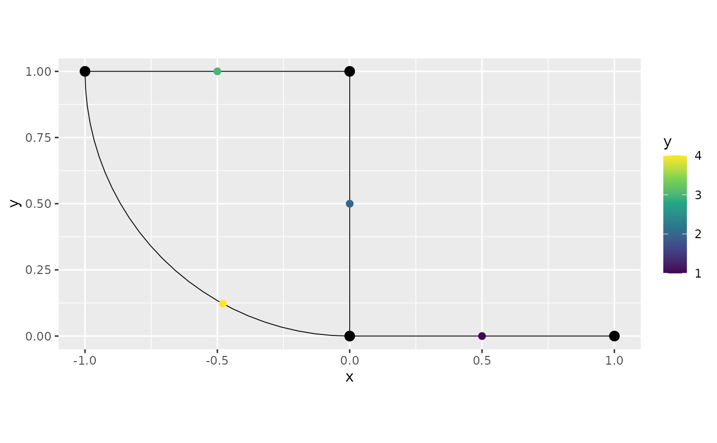
In certain situations, it might be easier to specify the relative
distances on the edges, so that 0 represents the start and 1 the end of
the edge (instead of the edge length). To do so, we can simply specify
normalized = TRUE when adding the observations. For
example, let us add one more observation at the midpoint of the fourth
edge:
obs.loc <- matrix(c(4, 0.5),1,2)
obs <- c(5)
df_new <- data.frame(y=obs, edge_number = obs.loc[,1],
distance_on_edge = obs.loc[,2])
graph$add_observations(data=df_new, normalized = TRUE)## Adding observations...## Assuming the observations are normalized by the length of the edge.
graph$plot(data = "y")
An alternative method is to specify the observations as spatial points objects, where the locations are given in Euclidean coordinates. In this case the observations are added to the closes location on the graph:
obs.loc <- rbind(c(0.7, 0), c(0, 0.2))
obs <- c(6,7)
points <- SpatialPointsDataFrame(coords = obs.loc,
data = data.frame(y = obs))
graph$add_observations(points)## Adding observations...## Converting data to PtE
graph$plot(data = "y")
If we want to replace the data in the object, we can use
clear_observations() to remove all current data:
graph$clear_observations()The metric_graph object can hold multiple variables of
data, and one can also specify a group argument that it
useful for specifying that data is grouped, which for example is the
case with data observed at different time points. As an example, let us
add two variables observed at two separate time points:
obs.loc <- cbind(c(1:4, 1:4), c(rep(0.5, 4), rep(0.7, 4)))
df_rep <- data.frame(y = c(1, 2, NA, 3, 4, 6, 5, 7),
x = c(NA, 8, 9, 10, 11, 12, 13, NA),
edge_number = obs.loc[,1],
distance_on_edge = obs.loc[,2],
time = c(rep(1, 4), rep(2, 4)))
graph$add_observations(data = df_rep, group = "time")## Adding observations...## Assuming the observations are NOT normalized by the length of the edge.If NA is given in some variable, this indicates that
this specific variable is not measured at that location and group. We
can now plot the individual variables by specifying their names in the
plot function together with the group number that we want to see. By
default the first group is shown.
graph$plot(data = "y", group = 2)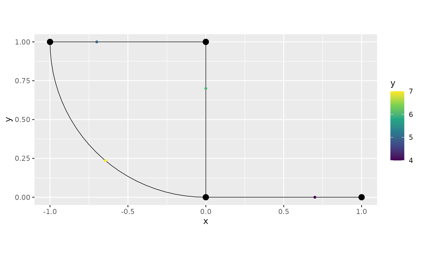
In some cases, we might want to add the observation locations as vertices in the graph. This can be done as follows:
graph$observation_to_vertex()
graph$plot(data = "x", group = 1)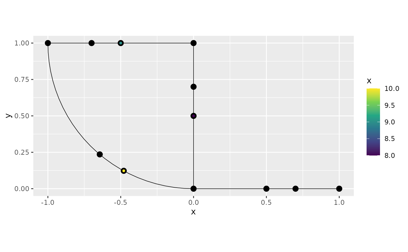
One can note that the command adds all observation locations, from all groups as vertices.
Finally, let us obtain a summary of the graph containing data:
summary(graph)## A metric graph object with:
##
## Vertices:
## Total: 12
## Degree 1: 1; Degree 2: 10; Degree 3: 1;
## With incompatible directions: 2
##
## Edges:
## Total: 12
## Lengths:
## Min: 0.2 ; Max: 0.8707963 ; Total: 4.570796
## Weights:
## Min: 1 ; Max: 1
## That are circles: 0
##
## Graph units:
## Vertices unit: None ; Lengths unit: None
##
## Longitude and Latitude coordinates: FALSE
##
## Some characteristics of the graph:
## Connected: TRUE
## Has loops: FALSE
## Has multiple edges: FALSE
## Is a tree: FALSE
## Distance consistent: TRUE
## Has Euclidean edges: TRUE
##
## Computed quantities inside the graph:
## Laplacian: FALSE ; Geodesic distances: TRUE
## Resistance distances: FALSE ; Finite element matrices: FALSE
##
## Mesh: The graph has no mesh!
##
## Data:
## Columns: y x time
## Groups: time
##
## Tolerances:
## vertex-vertex: 0.001
## vertex-edge: 0.001
## edge-edge: 0When dealing with SSN objects, one can also directly add
the SSN object as data:
river_graph$clear_observations()
river_graph$add_observations(data = mf04p)We can see that the data has been added correctly:
river_graph$get_data()## # A tibble: 45 × 32
## rid pid STREAMNAME COMID AREAWTMAP SLOPE ELEV_DEM Source Summer_mn
## <int> <int> <chr> <int> <dbl> <dbl> <int> <chr> <dbl>
## 1 1 3 Bear Valley 23519365 1001. 0.00274 1958 RMRS_M… 14.6
## 2 1 2 Bear Valley 23519365 1001. 0.00274 1952 RMRS_M… 14.7
## 3 1 1 Bear Valley 23519365 1001. 0.00274 1947 RMRS_M… 14.9
## 4 5 5 Bear Valley 23519297 1007. 0.00568 1932 RMRS_M… 14.5
## 5 5 4 Bear Valley 23519297 1007. 0.00568 1923 RMRS_M… 15.2
## 6 10 6 Bear Valley 23519307 1009. 0.00042 1940 RMRS_M… 15.3
## 7 13 7 Bear Valley 23519313 1010. 0 1940 RMRS_M… 15.1
## 8 15 8 Bear Valley 23519317 1013. 0.00297 1945 RMRS_M… 14.9
## 9 17 10 Elk 23519321 1025. 0 1950 RMRS_M… 15.0
## 10 17 9 Elk 23519321 1025. 0 1948 RMRS_M… 15.0
## # ℹ 35 more rows
## # ℹ 23 more variables: MaxOver20 <dbl>, C16 <dbl>, C20 <dbl>, C24 <dbl>,
## # FlowCMS <dbl>, AirMEANc <dbl>, AirMWMTc <dbl>, rcaAreaKm2 <dbl>,
## # h2oAreaKm2 <dbl>, ratio <dbl>, snapdist <dbl>, upDist <dbl>, afvArea <dbl>,
## # locID <int>, netID <dbl>, netgeom <chr>, .distance_to_graph <dbl>,
## # .edge_number <dbl>, .distance_on_edge <dbl>, .group <chr>, .loc_idx <int>,
## # .coord_x <dbl>, .coord_y <dbl>We can also plot the data:
river_graph$plot(data = "Summer_mn", vertex_size = 0.25)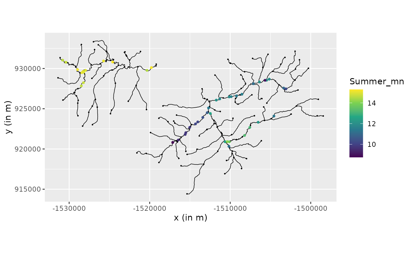
Let us clear the observations from the river graph:
river_graph$clear_observations()One can also directly add sf objects into the metric
graph. For example, the object mf04p$obs is an
sf object.
We can also add the obsevations as:
river_graph$add_observations(data = mf04p$obs)We can see that the observations have been added accordingly:
river_graph$get_data()## # A tibble: 45 × 32
## rid pid STREAMNAME COMID AREAWTMAP SLOPE ELEV_DEM Source Summer_mn
## <int> <int> <chr> <int> <dbl> <dbl> <int> <chr> <dbl>
## 1 1 3 Bear Valley 23519365 1001. 0.00274 1958 RMRS_M… 14.6
## 2 1 2 Bear Valley 23519365 1001. 0.00274 1952 RMRS_M… 14.7
## 3 1 1 Bear Valley 23519365 1001. 0.00274 1947 RMRS_M… 14.9
## 4 5 5 Bear Valley 23519297 1007. 0.00568 1932 RMRS_M… 14.5
## 5 5 4 Bear Valley 23519297 1007. 0.00568 1923 RMRS_M… 15.2
## 6 10 6 Bear Valley 23519307 1009. 0.00042 1940 RMRS_M… 15.3
## 7 13 7 Bear Valley 23519313 1010. 0 1940 RMRS_M… 15.1
## 8 15 8 Bear Valley 23519317 1013. 0.00297 1945 RMRS_M… 14.9
## 9 17 10 Elk 23519321 1025. 0 1950 RMRS_M… 15.0
## 10 17 9 Elk 23519321 1025. 0 1948 RMRS_M… 15.0
## # ℹ 35 more rows
## # ℹ 23 more variables: MaxOver20 <dbl>, C16 <dbl>, C20 <dbl>, C24 <dbl>,
## # FlowCMS <dbl>, AirMEANc <dbl>, AirMWMTc <dbl>, rcaAreaKm2 <dbl>,
## # h2oAreaKm2 <dbl>, ratio <dbl>, snapdist <dbl>, upDist <dbl>, afvArea <dbl>,
## # locID <int>, netID <dbl>, netgeom <chr>, .distance_to_graph <dbl>,
## # .edge_number <dbl>, .distance_on_edge <dbl>, .group <chr>, .loc_idx <int>,
## # .coord_x <dbl>, .coord_y <dbl>Working with functions on metric graphs
When working with data on metric graphs, one often wants to display
functions on the graph. The best way to visualize functions on the graph
is to evaluate them on a fine mesh over the graph and then use
plot_function. To illustrate this procedure, let us
consider the following graph:
V <- rbind(c(0, 0), c(1, 0), c(1, 1), c(0, 1), c(-1, 1), c(-1, 0), c(0, -1))
E <- rbind(c(1, 2), c(2, 3), c(3, 4), c(4, 5),
c(5, 6), c(6, 1), c(4, 1),c(1, 7))
graph <- metric_graph$new(V = V, E = E)
graph$build_mesh(h = 0.5)
graph$plot(mesh=TRUE)
In the command build_mesh, the argument h
decides the largest spacing between nodes in the mesh. As can be seen in
the plot, the mesh is very coarse, so let’s reduce the value of
h and rebuild the mesh:
graph$build_mesh(h = 0.01)Suppose now that we want to display the function
on this graph. We then first evaluate it on the vertices of the mesh and
then use the function plot_function to display it:
x <- graph$mesh$V[, 1]
y <- graph$mesh$V[, 2]
f <- x^2 - y^2
graph$plot_function(X = f)## Warning: The `X` argument of `plot_function()` is deprecated as of MetricGraph
## 1.3.0.9000.
## ℹ Please use the `newdata` argument instead.
## ℹ The argument `X` is deprecated; please use `newdata` to ensure the correct
## order when plotting.
## This warning is displayed once per session.
## Call `lifecycle::last_lifecycle_warnings()` to see where this warning was
## generated.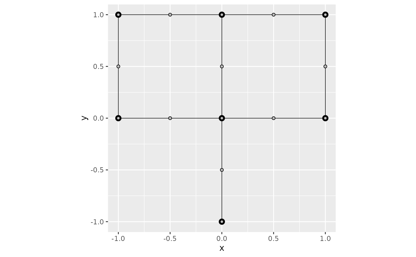
Alternatively, we can set type = "plotly" in the plot
command to get a 3D visualization of the function:
graph$plot_function(X = f, type = "plotly")When the first argument of plot_function is a vector,
the function assumes that the values in the vector are the values of the
function evaluated at the vertices of the mesh. As an alternative, one
can also provide a new dataset. To illustrate this, let us first
construct a set of locations that are evenly spaced over each edge.
Then, we will convert the data to Euclidean coordinates so that we can
evaluate the function above. Then, process the data and finally plot the
result:
n.e <- 30
PtE <- cbind(rep(1:graph$nE, each = n.e),
rep(seq(from = 0, to = 1, length.out = n.e), graph$nE))
XY <- graph$coordinates(PtE)
f <- XY[, 1]^2 - XY[, 2]^2
data_f <- data.frame(f = f, "edge_number" = PtE[,1],
"distance_on_edge" = PtE[,2])
data_f <- graph$process_data(data = data_f, normalized=TRUE)
graph$plot_function(data = "f", newdata = data_f, type = "plotly")Alternatively, we can add the data to the graph, and directly plot by
using the data argument. To illustration purposes, we will
build this next plot as a 2d plot:
graph$add_observations(data = data_f, clear_obs = TRUE, normalized = TRUE)## Adding observations...## Assuming the observations are normalized by the length of the edge.## Warning in graph$add_observations(data = data_f, clear_obs = TRUE, normalized =
## TRUE): There is at least one 'column' of the data with repeated (possibly
## different) values at the same location for the same group variable. Only one of
## these values will be used. Consider using the group variable to differentiate
## between these values or provide different names for such variables.
graph$plot_function(data = "f")
Further details on plot_function
By default, the values along the edges are interpolated try to
provide a better plot. This behavior can be disabled by setting
interpolate_plot to FALSE.
We begin by recreating the first graph we used in this vignette:
edge1 <- rbind(c(0,0),c(1,0))
edge2 <- rbind(c(0,0),c(0,1))
edge3 <- rbind(c(0,1),c(-1,1))
theta <- seq(from=pi,to=3*pi/2,length.out = 50)
edge4 <- cbind(sin(theta),1+ cos(theta))
edges = list(edge1, edge2, edge3, edge4)
graph <- metric_graph$new(edges = edges)Let us create a coarse mesh, so the interpolation can be easily seen.
graph$build_mesh(h=0.8)
graph$plot(mesh=TRUE)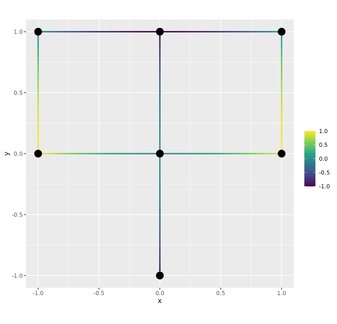
Let us compute the function the same function as before on this mesh:
XY <- graph$mesh$V
f <- XY[, 1]^2 - XY[, 2]^2We can directly plot from the mesh values. Let us start with the default, the interpolated plot:
graph$plot_function(f)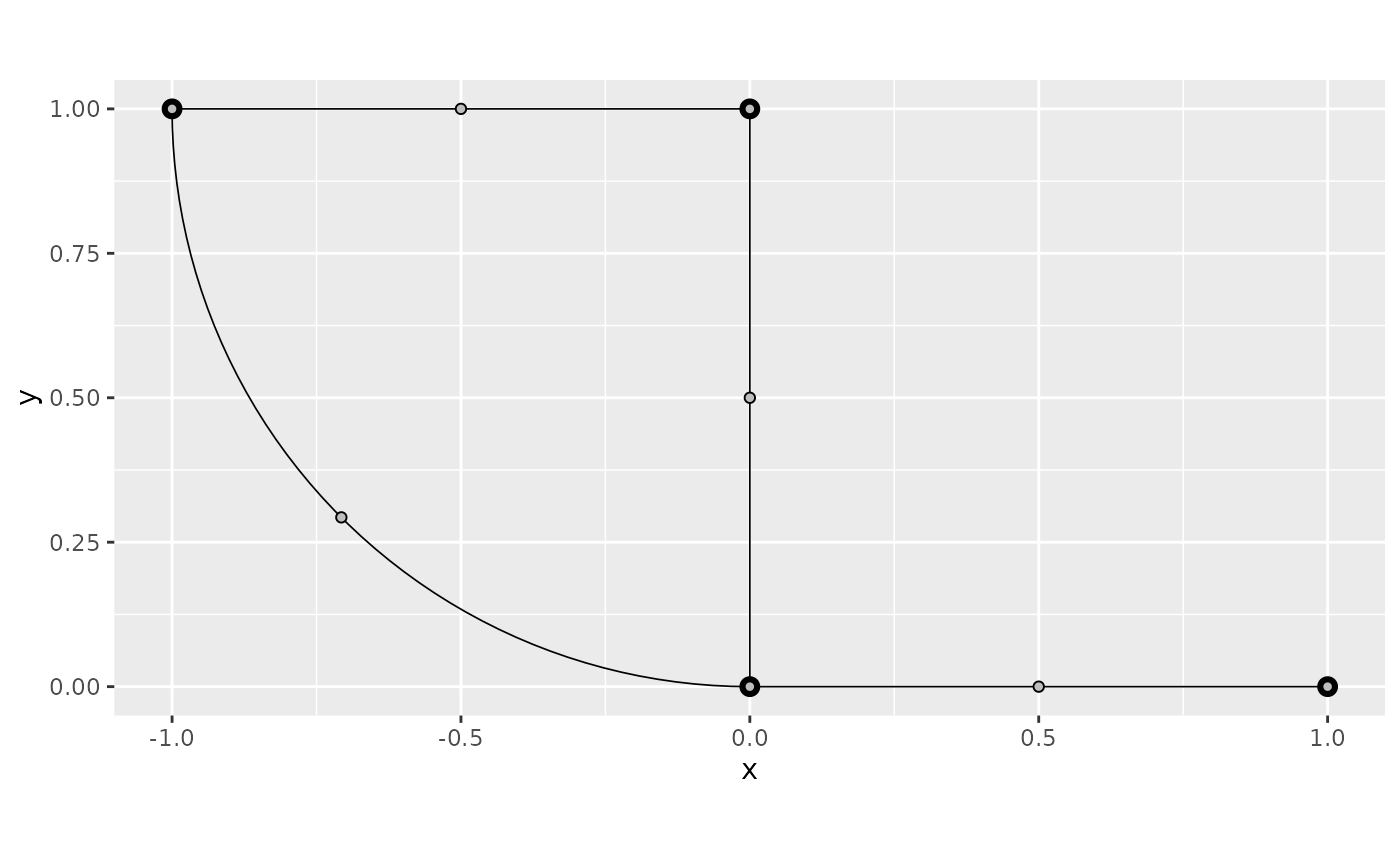
We can, now, turn off the interpolation by setting
interpolate_plot to FALSE:
graph$plot_function(f, interpolate_plot = FALSE)
Alternatively, we can supply the data through the
newdata argument. To such an end, we will need to supply
the data.frame. So let us build it:
df_f <- data.frame(edge_number = graph$mesh$VtE[,1],
distance_on_edge = graph$mesh$VtE[,2],
f = f)Let us now process the data.frame to the graph’s
internal data format using the process_data() method:
df_f <- graph$process_data(data = df_f, normalized=TRUE)We will now plot this function. First, let us do the default plot
from plot_function:
graph$plot_function(data = "f", newdata= df_f)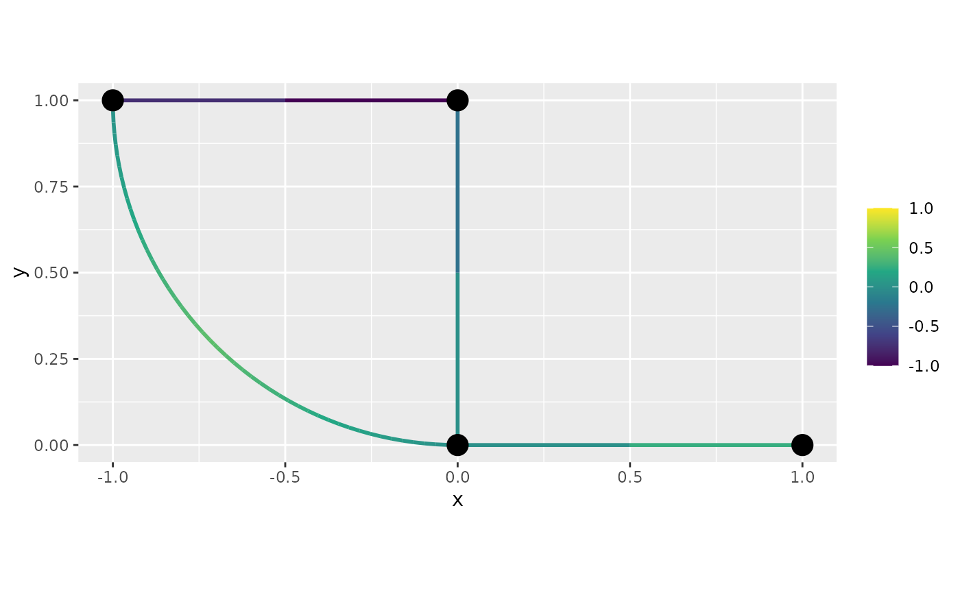
Let us now, create the same plot with
interpolate_plot=FALSE:
graph$plot_function(data = "f", newdata= df_f, interpolate_plot=FALSE)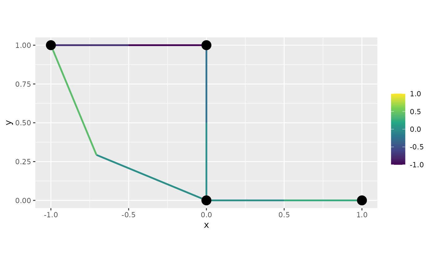
Let us now obtain a 3d plot. First, of the default version:
graph$plot_function(data = "f", newdata= df_f, type = "plotly")Now, of the non-interpolated version:
graph$plot_function(data = "f", newdata= df_f, type = "plotly",
interpolate_plot = FALSE)Note about continuity
However, it is important to observe that plot_function
assumes continuity of the function by default. Let us see an example of
a discontinuous function, and observe the effect of
plot_function.
For example, let us consider the function that takes the edge number (normalized). Let us also refine the mesh a bit, so it is easier to observe what is happening.
graph$build_mesh(h=0.2)
f <- graph$mesh$VtE[,1]/4Let us proceed with the creation of the data.frame and
processing of the data:
df_f <- data.frame(edge_number = graph$mesh$VtE[,1],
distance_on_edge = graph$mesh$VtE[,2],
f = f)
df_f <- graph$process_data(data = df_f, normalized=TRUE)We will now plot this function with the default plot from
plot_function:
graph$plot_function(data = "f", newdata= df_f)
Let us now, create the same plot with
interpolate_plot=FALSE:
graph$plot_function(data = "f", newdata= df_f, interpolate_plot=FALSE)
Let us now obtain a 3d plot. First, of the default version:
graph$plot_function(data = "f", newdata= df_f, type = "plotly")Now, of the non-interpolated version:
graph$plot_function(data = "f", newdata= df_f, type = "plotly",
interpolate_plot = FALSE)Observe that for both versions we have the same behavior around the vertices (which are the discontinuity points).
To work with discontinuous functions, the simplest option is to create a mesh that does not assume continuity:
graph$build_mesh(h=0.8, continuous = FALSE)In this mesh, each vertex is split into one vertex per edge connecting to the vertex, which allows for discontinuous functions.
f <- graph$mesh$PtE[,1]/4
graph$plot_function(f)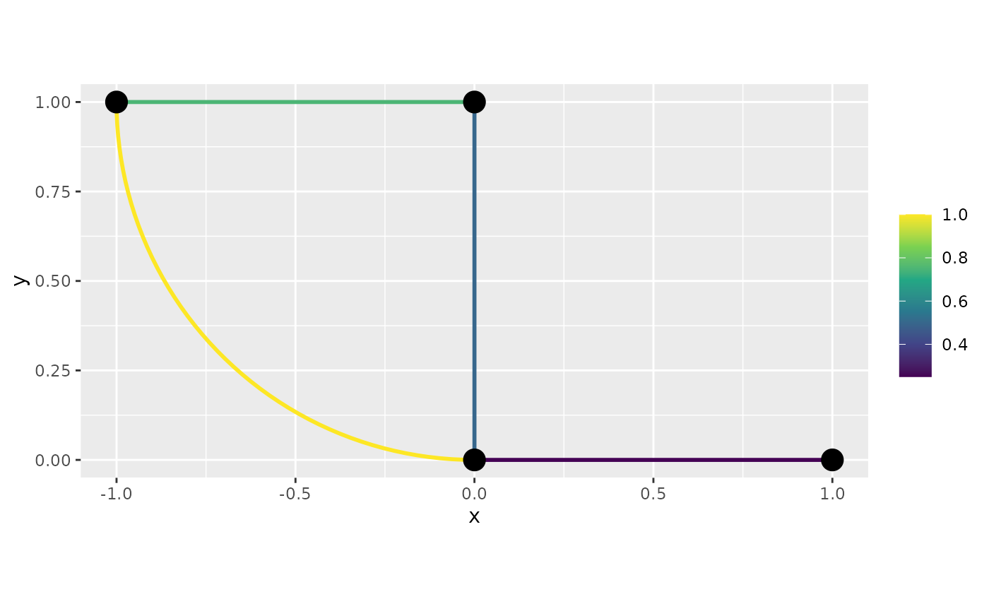
Similarly to the case for continuous meshes, we have the
interpolate_plot option:
graph$plot_function(f, interpolate_plot = FALSE)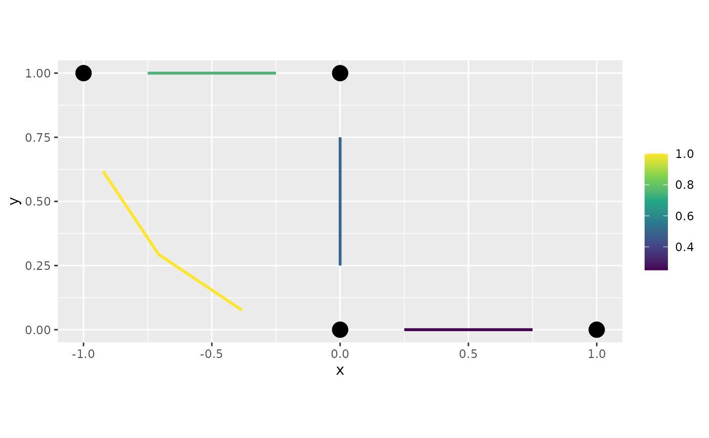
Now, the 3d plot:
graph$plot_function(f, type = "plotly", interpolate_plot = FALSE)Alternatively, we can similarly plot by setting the
data.frame and passing the newdata
argument:
df_f <- data.frame(edge_number = graph$mesh$VtE[,1],
distance_on_edge = graph$mesh$VtE[,2],
f = f)
df_f <- graph$process_data(data = df_f, normalized=TRUE)Let us now build the plots. In this case, we need to set the
continuous argument to FALSE. First the 2d
plot:
graph$plot_function(data = "f", newdata= df_f,
continuous = FALSE)
Now, the 3d plot:
graph$plot_function(data = "f", newdata= df_f, type = "plotly",
continuous = FALSE)