Data manipulation on metric graphs
David Bolin, Alexandre B. Simas, and Jonas Wallin
Created: 2023-10-24. Last modified: 2026-05-14.
Source:vignettes/metric_graph_data.Rmd
metric_graph_data.RmdIntroduction
In this vignette we will provide some examples of data manipulation
on metric graphs. More precisely, we will show how to add data to the
metric graph, how to retrieve the data, how to do data manipulation
using some of the tidyverse tools. Finally, we will show
how add the results of these manipulations back to the metric graph.
As an example throughout the vignette, we consider the following metric graph:
edge1 <- rbind(c(0,0),c(1,0))
edge2 <- rbind(c(0,0),c(0,1))
edge3 <- rbind(c(0,1),c(-1,1))
theta <- seq(from=pi,to=3*pi/2,length.out = 20)
edge4 <- cbind(sin(theta),1+ cos(theta))
edges = list(edge1, edge2, edge3, edge4)
graph <- metric_graph$new(edges = edges)
graph$plot()
For further details on the construction of metric graphs, see Working with metric graphs
Adding and accessing data on metric graphs
Let us start by generating some data to be added to the metric graph
object we created, namely graph. We first generate the
locations:
obs_per_edge <- 50
obs_loc <- NULL
for(i in 1:(graph$nE)) {
  obs_loc <- rbind(obs_loc,
                   cbind(rep(i,obs_per_edge),
                   runif(obs_per_edge)))
}
Now, we will generate the data and build a data.frame to
be added to the metric graph:
y <- rnorm(graph$nE * obs_per_edge)

df_data <- data.frame(y=y, edge = obs_loc[,1], pos = obs_loc[,2])
We can now add the data to the graph by using the
add_mesh_observations() method. We will add the data by
providing the edge number and relative distance on the edge. To this
end, when adding the data, we need to supply the names of the columns
that contain the edge number and the distance on edge by entering the
edge_number and distance_on_edge arguments.
Further, since we are providing the relative distance, we need to set
the normalized argument to TRUE:
graph$add_observations(data = df_data, edge_number = "edge",
                    distance_on_edge = "pos", normalized = TRUE)
## Adding observations...## Assuming the observations are normalized by the length of the edge.We can check that the data was successfully added by retrieving them
from the metric graph using the get_data() method:
graph$get_data()## # A tibble: 200 × 7
## y .edge_number .distance_on_edge .group .loc_idx .coord_x .coord_y
## <dbl> <dbl> <dbl> <chr> <int> <dbl> <dbl>
## 1 -0.0736 1 0.0134 1 1 0.0134 0
## 2 2.09 1 0.0233 1 2 0.0233 0
## 3 1.68 1 0.0618 1 3 0.0618 0
## 4 -0.528 1 0.108 1 4 0.108 0
## 5 -0.180 1 0.126 1 5 0.126 0
## 6 -0.462 1 0.177 1 6 0.177 0
## 7 -1.52 1 0.186 1 7 0.186 0
## 8 -0.655 1 0.202 1 8 0.202 0
## 9 -0.636 1 0.206 1 9 0.206 0
## 10 1.34 1 0.212 1 10 0.212 0
## # ℹ 190 more rowsWe can also visualize the data by using the plot()
method and specifying which column we would like to plot:
graph$plot(data = "y")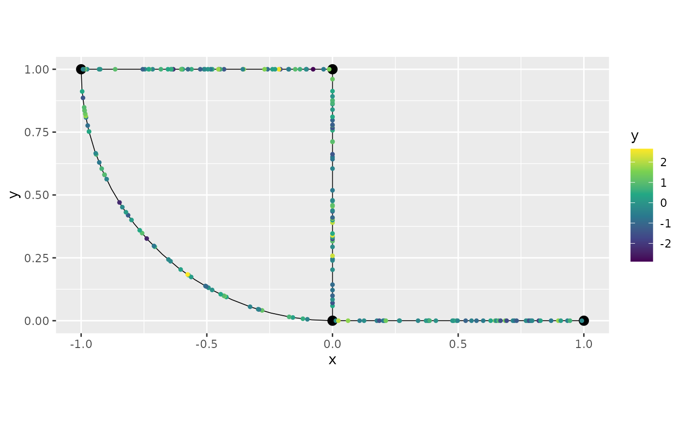
We can add more data to the metric graph by using the
add_observations() method again. To this end, let us create
an additional dataset. This time, we will add it using spatial
coordinates. In this case, we will generate 50 uniform
locations to be the x coordinate of the data, and we will
keep the y coordinate equal to zero. Further, we will
generate 50 more realizations of a standard gaussian
variable as the y2 variable.
coordx <- runif(50)
coordy <- 0
y2 <- rnorm(50)

df_data2 <- data.frame(y2 = y2, coordx = coordx, coordy = coordy)
Let us add this dataset. Now, we need to set data_coords
to "spatial" and we need to supply the names of the columns
of the x and y coordinates:
graph$add_observations(data = df_data2, data_coords = "spatial",
                            coord_x = "coordx", coord_y = "coordy")
## Adding observations...## Converting data to PtELet us check that the data was successfully added:
graph$get_data()## # A tibble: 250 × 9
## y y2 .distance_to_graph .edge_number .distance_on_edge .group
## <dbl> <dbl> <dbl> <dbl> <dbl> <chr>
## 1 -0.0736 NA NA 1 0.0134 1
## 2 2.09 NA NA 1 0.0233 1
## 3 NA 0.278 0 1 0.0308 1
## 4 NA -2.26 0 1 0.0574 1
## 5 1.68 NA NA 1 0.0618 1
## 6 NA -0.636 0 1 0.0649 1
## 7 NA 1.31 0 1 0.0978 1
## 8 NA -0.334 0 1 0.107 1
## 9 -0.528 NA NA 1 0.108 1
## 10 -0.180 NA NA 1 0.126 1
## # ℹ 240 more rows
## # ℹ 3 more variables: .loc_idx <int>, .coord_x <dbl>, .coord_y <dbl>We can also plot:
graph$plot(data = "y2")
Observe that NAs were added, since df_data
does not contain the column y2 and df_data2
does not contain the column y.
By default, the get_data() method excludes all rows in
which all the variables are NA (the location variables are
not considered here). We can also show the rows that do not contain any
NA observations by using the drop_na argument
in the get_data() method:
graph$get_data(drop_na = TRUE)## # A tibble: 0 × 9
## # ℹ 9 variables: y <dbl>, y2 <dbl>, .distance_to_graph <dbl>,
## # .edge_number <dbl>, .distance_on_edge <dbl>, .group <chr>, .loc_idx <int>,
## # .coord_x <dbl>, .coord_y <dbl>Observe that there is no row, since all of them contain at least one
NA.
Suppose now that we want to replace the metric graph data by a new
dataset. To this end we have two options. The first one is to use the
clear_observations() method, then add the observations:
graph$clear_observations()We will now create the dataset we want to add. To simplify, we will
use the default naming for the edge number and distance on edge, so that
we do not need to specify them in the add_observations()
method:
y3 <- rnorm(graph$nE * obs_per_edge)

df_data3 <- data.frame(y3=y3, edge_number = obs_loc[,1], distance_on_edge = obs_loc[,2])
We can now add the data. Remember to set normalized to
TRUE since we are providing the relative distance on
edge:
graph$add_observations(data = df_data3, normalized = TRUE)## Adding observations...## Assuming the observations are normalized by the length of the edge.and check:
graph$get_data()## # A tibble: 200 × 7
## y3 .edge_number .distance_on_edge .group .loc_idx .coord_x .coord_y
## <dbl> <dbl> <dbl> <chr> <int> <dbl> <dbl>
## 1 1.90 1 0.0134 1 1 0.0134 0
## 2 -0.710 1 0.0233 1 2 0.0233 0
## 3 1.15 1 0.0618 1 3 0.0618 0
## 4 1.12 1 0.108 1 4 0.108 0
## 5 -0.715 1 0.126 1 5 0.126 0
## 6 -2.13 1 0.177 1 6 0.177 0
## 7 1.44 1 0.186 1 7 0.186 0
## 8 1.76 1 0.202 1 8 0.202 0
## 9 -0.0565 1 0.206 1 9 0.206 0
## 10 1.59 1 0.212 1 10 0.212 0
## # ℹ 190 more rowsThe second way to replace the data in the metric graph is to set the
clear_obs argument to TRUE. We will also
create a new dataset using the default naming for the x and
y coordinates, so we do not need to specify them:
df_data4 <- data.frame(y4 = exp(y2), coord_x = coordx, coord_y = coordy)and we add them (remember to set data_coords to
"spatial"):
graph$add_observations(data = df_data4, clear_obs = TRUE,
                            data_coords = "spatial")
## Adding observations...## Converting data to PtEand we can check it replaced:
graph$get_data()## # A tibble: 50 × 8
## y4 .distance_to_graph .edge_number .distance_on_edge .group .loc_idx
## <dbl> <dbl> <dbl> <dbl> <chr> <int>
## 1 1.32 0 1 0.0308 1 1
## 2 0.104 0 1 0.0574 1 2
## 3 0.530 0 1 0.0649 1 3
## 4 3.72 0 1 0.0978 1 4
## 5 0.716 0 1 0.107 1 5
## 6 2.23 0 1 0.136 1 6
## 7 1.19 0 1 0.147 1 7
## 8 0.345 0 1 0.153 1 8
## 9 0.564 0 1 0.202 1 9
## 10 2.50 0 1 0.213 1 10
## # ℹ 40 more rows
## # ℹ 2 more variables: .coord_x <dbl>, .coord_y <dbl>Adding grouped data to metric graphs
The graph structure also allow to add grouped data. To this end we need to specify which column of the data will be the grouping variable.
To illustrate, let us generate a grouped data. We will use the same locations we generated in the previous section.
n.repl <- 5

y_repl <- rnorm(n.repl * graph$nE * obs_per_edge)
repl <- rep(1:n.repl, each = graph$nE * obs_per_edge)
Let us now create the data.frame with the grouped data,
where the grouping variable is repl:
df_data_repl <- data.frame(y = y_repl, repl = repl,
                  edge_number = rep(obs_loc[,1], times = n.repl),
                  distance_on_edge = rep(obs_loc[,2], times = n.repl))
We can now add this data.frame to the graph by using the
add_observations() method. We need to set
normalized to TRUE, since we have relative
distances on edge. We also need to set the group argument
to repl, since repl is our grouping variable.
Finally, we will also set clear_obs to TRUE
since we want to replace the existing data.
graph$add_observations(data = df_data_repl,
                        normalized = TRUE,
                        clear_obs = TRUE,
                        group = "repl")
## Adding observations...## Assuming the observations are normalized by the length of the edge.Let us check the graph data. Observe that the grouping variable is
now .group.
graph$get_data()## # A tibble: 1,000 × 8
## y repl .edge_number .distance_on_edge .group .loc_idx .coord_x .coord_y
## <dbl> <int> <dbl> <dbl> <chr> <int> <dbl> <dbl>
## 1 1.50 1 1 0.0134 1 1 0.0134 0
## 2 -1.79 1 1 0.0233 1 2 0.0233 0
## 3 0.488 1 1 0.0618 1 3 0.0618 0
## 4 -0.385 1 1 0.108 1 4 0.108 0
## 5 0.905 1 1 0.126 1 5 0.126 0
## 6 -0.145 1 1 0.177 1 6 0.177 0
## 7 2.00 1 1 0.186 1 7 0.186 0
## 8 -1.16 1 1 0.202 1 8 0.202 0
## 9 0.879 1 1 0.206 1 9 0.206 0
## 10 -0.816 1 1 0.212 1 10 0.212 0
## # ℹ 990 more rowsWe can obtain the data for a given group by setting the
group argument in the get_data() method:
graph$get_data(group = "3")## # A tibble: 200 × 8
## y repl .edge_number .distance_on_edge .group .loc_idx .coord_x
## <dbl> <int> <dbl> <dbl> <chr> <int> <dbl>
## 1 1.11 3 1 0.0134 3 1 0.0134
## 2 0.774 3 1 0.0233 3 2 0.0233
## 3 0.464 3 1 0.0618 3 3 0.0618
## 4 -1.62 3 1 0.108 3 4 0.108
## 5 -1.48 3 1 0.126 3 5 0.126
## 6 -0.815 3 1 0.177 3 6 0.177
## 7 -1.25 3 1 0.186 3 7 0.186
## 8 0.0646 3 1 0.202 3 8 0.202
## 9 0.129 3 1 0.206 3 9 0.206
## 10 -0.881 3 1 0.212 3 10 0.212
## # ℹ 190 more rows
## # ℹ 1 more variable: .coord_y <dbl>We can also provide the group argument as a vector:
graph$get_data(group = c("3","5"))## # A tibble: 400 × 8
## y repl .edge_number .distance_on_edge .group .loc_idx .coord_x
## <dbl> <int> <dbl> <dbl> <chr> <int> <dbl>
## 1 1.11 3 1 0.0134 3 1 0.0134
## 2 0.774 3 1 0.0233 3 2 0.0233
## 3 0.464 3 1 0.0618 3 3 0.0618
## 4 -1.62 3 1 0.108 3 4 0.108
## 5 -1.48 3 1 0.126 3 5 0.126
## 6 -0.815 3 1 0.177 3 6 0.177
## 7 -1.25 3 1 0.186 3 7 0.186
## 8 0.0646 3 1 0.202 3 8 0.202
## 9 0.129 3 1 0.206 3 9 0.206
## 10 -0.881 3 1 0.212 3 10 0.212
## # ℹ 390 more rows
## # ℹ 1 more variable: .coord_y <dbl>The plot() method works similarly. We can plot the data
from a specific group by specifying which group we would like to
plot:
graph$plot(data = "y", group = "3")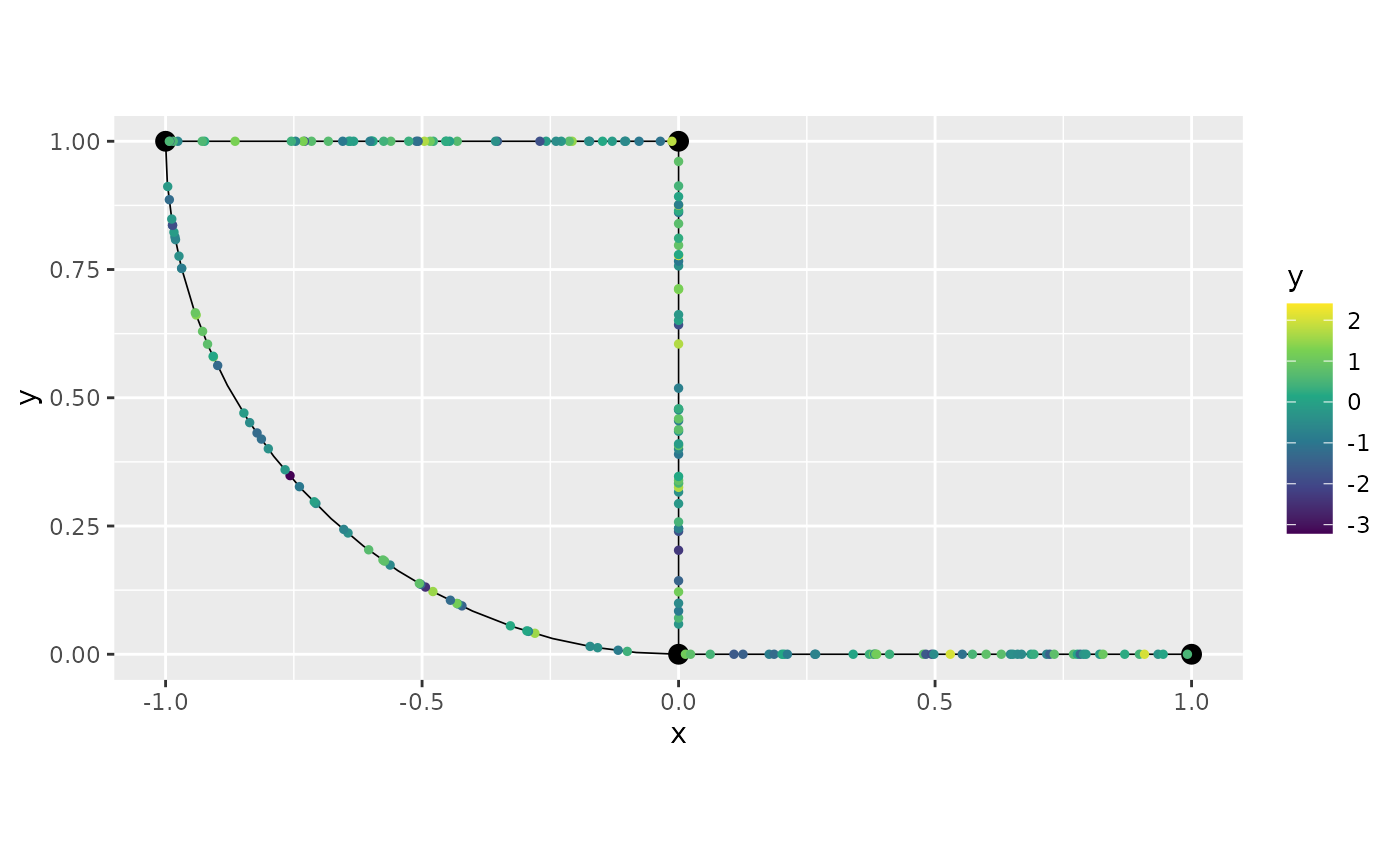
More advanced grouping
Besides being able to group data acoording to one column of the data, we can also group the data with respect to several columns of the data. Let us generate a new data set:
n.repl <- 10

y_repl <- rnorm(n.repl * graph$nE * obs_per_edge)
repl_1 <- rep(1:n.repl, each = graph$nE * obs_per_edge)
repl_2 <- rep(c("a","b","c","d","e"), times = 2 * graph$nE * obs_per_edge)

df_adv_grp <- data.frame(data.frame(y = y_repl,
                  repl_1 = repl_1, repl_2 = repl_2,
                  edge_number = rep(obs_loc[,1], times = n.repl),
                  distance_on_edge = rep(obs_loc[,2], times = n.repl)))
Let us now add these observations on the graph and group them by
c("repl_1","repl_2"):
graph$add_observations(data = df_adv_grp,
                        normalized = TRUE,
                        clear_obs = TRUE,
                        group = c("repl_1", "repl_2"))
## Adding observations...## Assuming the observations are normalized by the length of the edge.Let us take a look at the grouped variables. They are stored in the
.group column:
graph$get_data()## # A tibble: 2,000 × 9
## y repl_1 repl_2 .edge_number .distance_on_edge .group .loc_idx .coord_x
## <dbl> <int> <chr> <dbl> <dbl> <chr> <int> <dbl>
## 1 1.15 1 a 1 0.206 1.a 9 0.206
## 2 -0.529 1 a 1 0.266 1.a 11 0.266
## 3 0.344 1 a 1 0.386 1.a 18 0.386
## 4 0.921 1 a 1 0.482 1.a 21 0.482
## 5 -0.626 1 a 1 0.498 1.a 23 0.498
## 6 0.760 1 a 1 0.668 1.a 32 0.668
## 7 0.101 1 a 1 0.789 1.a 41 0.789
## 8 1.31 1 a 1 0.821 1.a 43 0.821
## 9 -1.35 1 a 1 0.898 1.a 46 0.898
## 10 -1.05 1 a 1 0.935 1.a 48 0.935
## # ℹ 1,990 more rows
## # ℹ 1 more variable: .coord_y <dbl>Observe that the group variable is created, by default,
by pasting the group variables together with the . as
separator. We can change the separator using the group_sep
argument:
graph$add_observations(data = df_adv_grp,
                        normalized = TRUE,
                        clear_obs = TRUE,
                        group = c("repl_1", "repl_2"),
                        group_sep = ":")
## Adding observations...## Assuming the observations are normalized by the length of the edge.Then,
graph$get_data()## # A tibble: 2,000 × 9
## y repl_1 repl_2 .edge_number .distance_on_edge .group .loc_idx .coord_x
## <dbl> <int> <chr> <dbl> <dbl> <chr> <int> <dbl>
## 1 1.15 1 a 1 0.206 1:a 9 0.206
## 2 -0.529 1 a 1 0.266 1:a 11 0.266
## 3 0.344 1 a 1 0.386 1:a 18 0.386
## 4 0.921 1 a 1 0.482 1:a 21 0.482
## 5 -0.626 1 a 1 0.498 1:a 23 0.498
## 6 0.760 1 a 1 0.668 1:a 32 0.668
## 7 0.101 1 a 1 0.789 1:a 41 0.789
## 8 1.31 1 a 1 0.821 1:a 43 0.821
## 9 -1.35 1 a 1 0.898 1:a 46 0.898
## 10 -1.05 1 a 1 0.935 1:a 48 0.935
## # ℹ 1,990 more rows
## # ℹ 1 more variable: .coord_y <dbl>To plot the data for a particular group, we simply select the group
variable we want to plot. Let us plot y for
repl_1 equal to 3 and repl_2
equal to c:
graph$plot(data = "y", group = "3:c")
Identifying data that is away from the metric graph
Whenever we use the add_observations() method, it
returns the data that was removed (if there was any). We can use this
information to visualize what is going on and decide what to do with
this data. There are two types of removed data, the ones that were
removed due to being projected to the same place, or the ones that were
removed due to being farther than the tolerance.
To make things simple, let us work with the previous dataset:
data_df <- as.data.frame(graph$get_data(group = "1:a"))
data_df <- data_df[,c("y", ".coord_x", ".coord_y")]
Let us now include observations that are not contained in the graph.
data_df_tmp <- data.frame(y = rnorm(20), .coord_x = 0.5, .coord_y = runif(20))
data_df <- rbind(data_df,data_df_tmp)
We start by looking at the graph, and the observations that we created outside the metric graph:
library(ggplot2)
graph$plot() + geom_point(data_df_tmp, mapping = aes(x=.coord_x, y=.coord_y), color="red")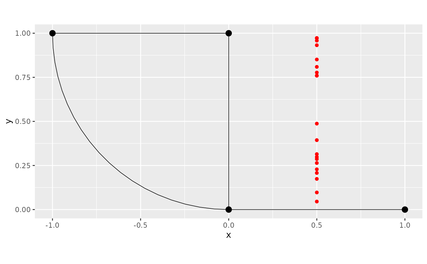
Let us now add these observations to the graph, but we will store the returned object:
rem_obs <- graph$add_observations(data = data_df, clear_obs = TRUE,
                                  data_coords = "spatial",
                                  coord_x = ".coord_x",
                                  coord_y = ".coord_y")
## Adding observations...## Converting data to PtE## Warning in system.time({: There were points projected at the same location.
## Only the closest point was kept. To keep all the observations change
## 'duplicated_strategy' to 'jitter'.Let us look at the element rem_obs:
rem_obs## $removed
## y .coord_x .coord_y
## 1 0.4232452 0.5 0.29823745
## 2 -0.5192331 0.5 0.26404506
## 3 -1.2447383 0.5 0.09702358
## 4 -0.1604400 0.5 0.17389470
## 5 1.0215809 0.5 0.48740037
## 6 -0.2034348 0.5 0.28642464
## 7 0.4112782 0.5 0.22832722
## 8 -1.0145804 0.5 0.39375818
## 9 -1.6322899 0.5 0.31439710
## 10 -0.2341612 0.5 0.20753836We can see that there were only data that were removed due to being projected at the same location.
Let us now plot the data, and add the points that were removed in red:
graph$plot(data = "y") + geom_point(rem_obs$removed, mapping = aes(x=.coord_x, y=.coord_y), color="red")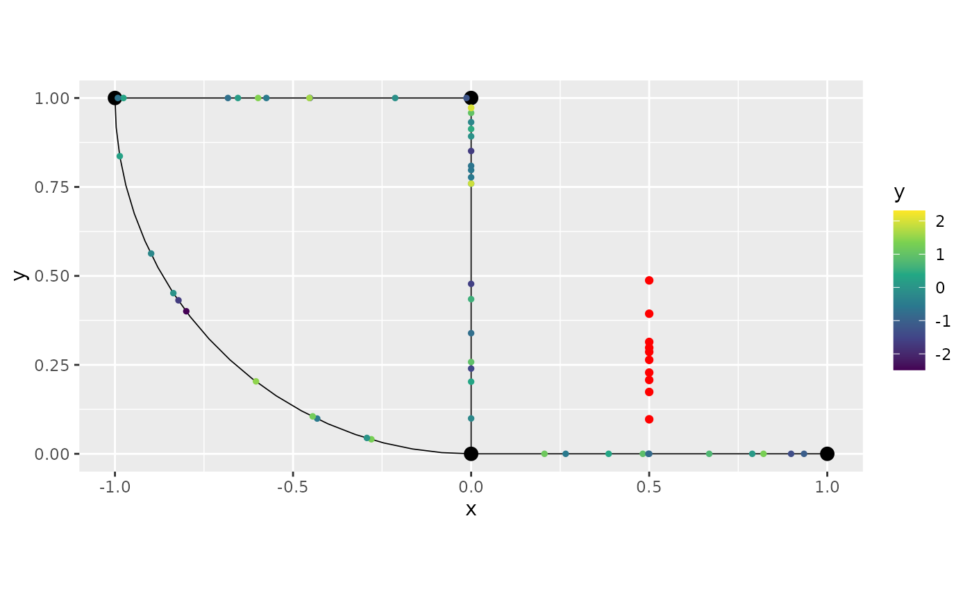
We can observe that we ended up adding more than one would want due to the tolerance for adding observations in this case. Let us reduce the tolerance, and repeat the procedure:
rem_obs <- graph$add_observations(data = data_df, clear_obs = TRUE,
                                  data_coords = "spatial",
                                  coord_x = ".coord_x",
                                  coord_y = ".coord_y",
                                  tolerance = 0.1)
## Adding observations...## Converting data to PtE## Warning in system.time({: There were points projected at the same location.
## Only the closest point was kept. To keep all the observations change
## 'duplicated_strategy' to 'jitter'.## Warning in system.time({: There were points that were farther than the
## tolerance. These points were removed. If you want them projected into the
## graph, please increase the tolerance. The total number of points removed due do
## being far is 18Let us now look at rem_obs:
rem_obs## $removed
## y .coord_x .coord_y
## 1 -1.244738 0.5 0.09702358
##
## $far_data
## y .coord_x .coord_y
## 1 0.4232452 0.5 0.2982374
## 2 -0.5192331 0.5 0.2640451
## 3 1.9191114 0.5 0.7595126
## 4 -0.1604400 0.5 0.1738947
## 5 1.0215809 0.5 0.4874004
## 6 -0.6328309 0.5 0.8092854
## 7 -0.2034348 0.5 0.2864246
## 8 0.4112782 0.5 0.2283272
## 9 -1.0145804 0.5 0.3937582
## 10 0.9982877 0.5 0.9581020
## 11 -1.6322899 0.5 0.3143971
## 12 -0.2341612 0.5 0.2075384
## 13 -1.6551095 0.5 0.8510350
## 14 2.3088834 0.5 0.9720656
## 15 -0.2635556 0.5 0.9320120
## 16 1.9971085 0.5 0.9729072
## 17 -0.2428420 0.5 0.7591693
## 18 -0.5547395 0.5 0.7771089We can see that there were both data removed due to being projected to the same place, as well as due to being too far away. Let us plot the ones due to being projected to the same place in red, and the ones that are far away in blue:
Let us now plot the data, and add the points that were removed in red:
graph$plot(data = "y") + geom_point(rem_obs$removed, mapping = aes(x=.coord_x, y=.coord_y), color="red") +
    geom_point(rem_obs$far_data, mapping = aes(x=.coord_x, y=.coord_y), color="blue")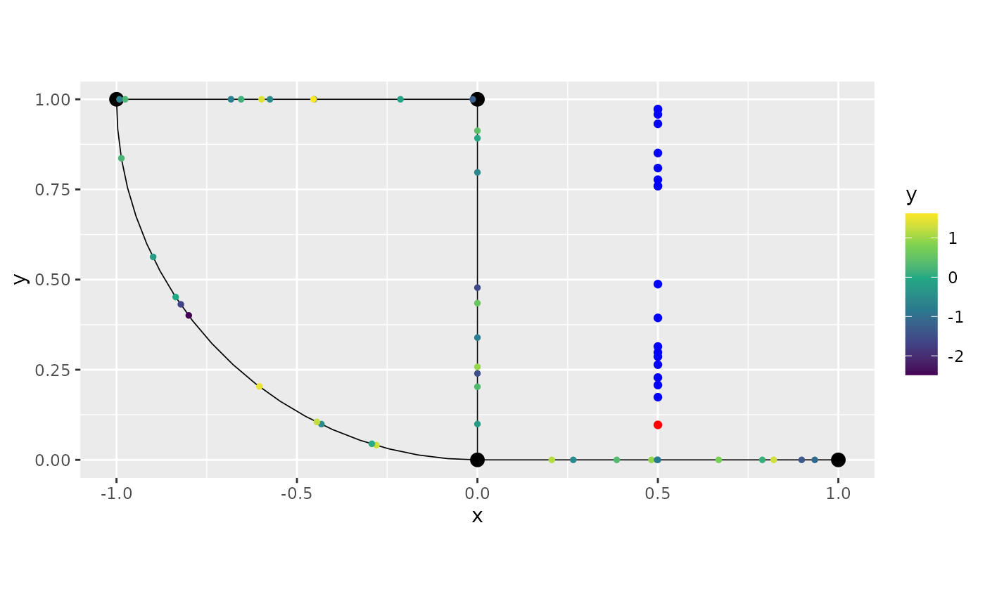
Therefore, the practitioner can use this information, to decide the best strategy to handle such observations.
Merging observations when adding them
Let us now consider the situation in which we have observations very
close, which can sometimes might lead to instabilities when fitting
models. By default nothing is done is this case. To handle such cases,
we have the tolerance_merge argument, for which
observations on a common edge within this tolerance will be merged, for
which the default value is 0. We have three alternative
strategies: remove, merge and
average. These can be set by using the
merge_strategy argument.
It is also important to note that, by default, the removed
observations due to merge will be returned from the
add_observations() call.
Let us illustrate with a simple example. First, with the merge
strategy set to merge. For this strategy, the observations
will be merged by filling the NA columns of the
observations within the tolerance region, by some non-NA value from an
observation within the same tolerance region.
Let us create a simple data.frame with some observations
that are close to each other:
df_graph <- data.frame(
    y = c(NA, 2, 3, 4, 1, 10),
    edge_number = c(1, 2, 3, 4, 1, 2),
    distance_on_edge = c(0.5, 0.5, 0.5, 0.5, 0.449, 0.45),
    z = c(10, NA, 30, 40, NA, 60),
    w = c("a", "b", "c", "d", "e", NA)
)

graph$add_observations(data = df_graph, normalized = TRUE, clear_obs = TRUE)
## Adding observations...## Assuming the observations are normalized by the length of the edge.let us look at the data
graph$get_data()## # A tibble: 6 × 9
## y z w .edge_number .distance_on_edge .group .loc_idx .coord_x
## <dbl> <dbl> <chr> <dbl> <dbl> <chr> <int> <dbl>
## 1 1 NA e 1 0.449 1 1 0.449
## 2 NA 10 a 1 0.5 1 2 0.5
## 3 10 60 NA 2 0.45 1 3 0
## 4 2 NA b 2 0.5 1 4 0
## 5 3 30 c 3 0.5 1 5 -0.5
## 6 4 40 d 4 0.5 1 6 -0.707
## # ℹ 1 more variable: .coord_y <dbl>We will merge these observations, with the removal strategy, by
setting tolerance_merge to 0.1:
graph$add_observations(data = df_graph, normalized = TRUE, clear_obs = TRUE,
                        merge_strategy = "merge", tolerance_merge = 0.1)
## Adding observations...## Assuming the observations are normalized by the length of the edge.## $removed_merge
## y z w .edge_number .distance_on_edge
## 1 NA 10 a 1 0.5
## 2 2 NA b 2 0.5We can see from the output that the merged observations were returned. Now, let us look at the data added to the graph with this merge strategy:
graph$get_data()## # A tibble: 4 × 9
## y z w .edge_number .distance_on_edge .group .loc_idx .coord_x
## <dbl> <dbl> <chr> <dbl> <dbl> <chr> <int> <dbl>
## 1 1 10 e 1 0.449 1 1 0.449
## 2 10 60 b 2 0.45 1 2 0
## 3 3 30 c 3 0.5 1 3 -0.5
## 4 4 40 d 4 0.5 1 4 -0.707
## # ℹ 1 more variable: .coord_y <dbl>We can observe that the NA values were filled by the
ones from the observations within the same tolerance region.
Now, let us see the remove strategy. For this strategy,
the observations that are within the tolerance from each other will be
removed, keeping only one observation per “tolerance region”.
graph$add_observations(data = df_graph, normalized = TRUE, clear_obs = TRUE,
                        merge_strategy = "remove", tolerance_merge = 0.1)
## Adding observations...## Assuming the observations are normalized by the length of the edge.## $removed_merge
## y z w .edge_number .distance_on_edge
## 1 NA 10 a 1 0.5
## 2 2 NA b 2 0.5We can see the removed observations due to merge, now let us check the added observations:
graph$get_data()## # A tibble: 4 × 9
## y z w .edge_number .distance_on_edge .group .loc_idx .coord_x
## <dbl> <dbl> <chr> <dbl> <dbl> <chr> <int> <dbl>
## 1 1 NA e 1 0.449 1 1 0.449
## 2 10 60 NA 2 0.45 1 2 0
## 3 3 30 c 3 0.5 1 3 -0.5
## 4 4 40 d 4 0.5 1 4 -0.707
## # ℹ 1 more variable: .coord_y <dbl>We can see that the observations that were within the tolerance
region were removed, and the added observations did not have their
NA values filled in. So, it was a simple removal of
observations within the same tolerance region.
Finally, let us look at the average merge strategy. For
this strategy, the non-NA values of numerical columns of observations
that are within the tolerance from each other will be averaged, keeping
only one observation per “tolerance region”. But for non-numerical
columns, the behavior is identical to the merge strategy,
that is, if the column has a non-NA value, it will be kept as is, but if
it has an NA value, a search for a non-NA value will be performed across
the observations within the tolerance region. Let us illustrate
this:
graph$add_observations(data = df_graph, normalized = TRUE, clear_obs = TRUE,
                        merge_strategy = "average", tolerance_merge = 0.1)
## Adding observations...## Assuming the observations are normalized by the length of the edge.## $removed_merge
## y z w .edge_number .distance_on_edge
## 1 NA 10 a 1 0.5
## 2 2 NA b 2 0.5Observe that the removed observations due to merge were returned. Now, let us look at the data inside the graph:
graph$get_data()## # A tibble: 4 × 9
## y z w .edge_number .distance_on_edge .group .loc_idx .coord_x
## <dbl> <dbl> <chr> <dbl> <dbl> <chr> <int> <dbl>
## 1 1 10 e 1 0.449 1 1 0.449
## 2 6 60 b 2 0.45 1 2 0
## 3 3 30 c 3 0.5 1 3 -0.5
## 4 4 40 d 4 0.5 1 4 -0.707
## # ℹ 1 more variable: .coord_y <dbl>We can observe that for columns z and w,
the NA values were filled by the ones from the observations
within the same tolerance region. However, for column y,
the non-NA values were averaged.
Manipulating data from metric graphs in the tidyverse style
In this section we will present some data manipulation tools that are implemented in metric graphs and can be safely used.
The tools are based on dplyr::select(),
dplyr::mutate(), dplyr::filter(),
dplyr::summarise() and tidyr::drop_na().
Let us generate a dataset that will be widely used throughout this
section and add this to the metric graph object. Observe that we are
replacing the existing data by setting clear_obs to
TRUE:
df_tidy <- data.frame(y=y, y2 = exp(y), y3 = y^2, y4 = sin(y),
       edge_number = obs_loc[,1], distance_on_edge = obs_loc[,2])

# Ordering to simplify presentation with NA data
ord_idx <- order(df_tidy[["edge_number"]],
                df_tidy[["distance_on_edge"]])
df_tidy <- df_tidy[ord_idx,]

# Setting some NA data
df_tidy[["y"]][1] <- df_tidy[["y2"]][1] <- NA
df_tidy[["y3"]][1] <- df_tidy[["y4"]][1] <- NA

df_tidy[["y2"]][2] <- NA
df_tidy[["y3"]][3] <- NA

graph$add_observations(data = df_tidy, clear_obs = TRUE, normalized = TRUE)
## Adding observations...## Assuming the observations are normalized by the length of the edge.Let us look at the complete data:
graph$get_data(drop_all_na = FALSE)## # A tibble: 200 × 10
## y y2 y3 y4 .edge_number .distance_on_edge .group .loc_idx
## <dbl> <dbl> <dbl> <dbl> <dbl> <dbl> <chr> <int>
## 1 NA NA NA NA 1 0.0134 1 1
## 2 2.09 NA 4.36 0.870 1 0.0233 1 2
## 3 1.68 5.38 NA 0.994 1 0.0618 1 3
## 4 -0.528 0.590 0.279 -0.504 1 0.108 1 4
## 5 -0.180 0.836 0.0322 -0.179 1 0.126 1 5
## 6 -0.462 0.630 0.213 -0.445 1 0.177 1 6
## 7 -1.52 0.219 2.31 -0.999 1 0.186 1 7
## 8 -0.655 0.520 0.428 -0.609 1 0.202 1 8
## 9 -0.636 0.530 0.404 -0.594 1 0.206 1 9
## 10 1.34 3.83 1.80 0.974 1 0.212 1 10
## # ℹ 190 more rows
## # ℹ 2 more variables: .coord_x <dbl>, .coord_y <dbl>select
The verb select allows one to choose which columns to
keep or to remove.
For example, let us select the columns y and
y2 from the metric graph dataset using the
select() method:
graph$select(y,y2)## # A tibble: 199 × 7
## y y2 .group .edge_number .distance_on_edge .coord_x .coord_y
## <dbl> <dbl> <chr> <dbl> <dbl> <dbl> <dbl>
## 1 2.09 NA 1 1 0.0233 0.0233 0
## 2 1.68 5.38 1 1 0.0618 0.0618 0
## 3 -0.528 0.590 1 1 0.108 0.108 0
## 4 -0.180 0.836 1 1 0.126 0.126 0
## 5 -0.462 0.630 1 1 0.177 0.177 0
## 6 -1.52 0.219 1 1 0.186 0.186 0
## 7 -0.655 0.520 1 1 0.202 0.202 0
## 8 -0.636 0.530 1 1 0.206 0.206 0
## 9 1.34 3.83 1 1 0.212 0.212 0
## 10 -0.620 0.538 1 1 0.266 0.266 0
## # ℹ 189 more rowsFirst, observe that this select verb is metric graph
friendly since it does not remove the columns related to spatial
locations.
Also observe that the first original row, that contains only
NA was removed by default. To return all the rows, we can
set the argument .drop_all_na to FALSE:
graph$select(y, y2, .drop_all_na = FALSE)## # A tibble: 200 × 7
## y y2 .group .edge_number .distance_on_edge .coord_x .coord_y
## <dbl> <dbl> <chr> <dbl> <dbl> <dbl> <dbl>
## 1 NA NA 1 1 0.0134 0.0134 0
## 2 2.09 NA 1 1 0.0233 0.0233 0
## 3 1.68 5.38 1 1 0.0618 0.0618 0
## 4 -0.528 0.590 1 1 0.108 0.108 0
## 5 -0.180 0.836 1 1 0.126 0.126 0
## 6 -0.462 0.630 1 1 0.177 0.177 0
## 7 -1.52 0.219 1 1 0.186 0.186 0
## 8 -0.655 0.520 1 1 0.202 0.202 0
## 9 -0.636 0.530 1 1 0.206 0.206 0
## 10 1.34 3.83 1 1 0.212 0.212 0
## # ℹ 190 more rowsFurther, observe that the second row also contain an NA
value in y2. To remove all the rows that contain
NA for at least one variable, we can set the argument
.drop_na to TRUE:
graph$select(y, y2, .drop_na = TRUE)## # A tibble: 198 × 7
## y y2 .group .edge_number .distance_on_edge .coord_x .coord_y
## <dbl> <dbl> <chr> <dbl> <dbl> <dbl> <dbl>
## 1 1.68 5.38 1 1 0.0618 0.0618 0
## 2 -0.528 0.590 1 1 0.108 0.108 0
## 3 -0.180 0.836 1 1 0.126 0.126 0
## 4 -0.462 0.630 1 1 0.177 0.177 0
## 5 -1.52 0.219 1 1 0.186 0.186 0
## 6 -0.655 0.520 1 1 0.202 0.202 0
## 7 -0.636 0.530 1 1 0.206 0.206 0
## 8 1.34 3.83 1 1 0.212 0.212 0
## 9 -0.620 0.538 1 1 0.266 0.266 0
## 10 -0.100 0.905 1 1 0.267 0.267 0
## # ℹ 188 more rowsMoreover, if we want to remove a column, we can simply use the
select() method together with adding a minus sign
- in front of the column we want to be removed. For
example, to remove y2, we can do:
graph$select(-y2)## # A tibble: 200 × 9
## y y3 y4 .edge_number .distance_on_edge .group .loc_idx .coord_x
## <dbl> <dbl> <dbl> <dbl> <dbl> <chr> <int> <dbl>
## 1 NA NA NA 1 0.0134 1 1 0.0134
## 2 2.09 4.36 0.870 1 0.0233 1 2 0.0233
## 3 1.68 NA 0.994 1 0.0618 1 3 0.0618
## 4 -0.528 0.279 -0.504 1 0.108 1 4 0.108
## 5 -0.180 0.0322 -0.179 1 0.126 1 5 0.126
## 6 -0.462 0.213 -0.445 1 0.177 1 6 0.177
## 7 -1.52 2.31 -0.999 1 0.186 1 7 0.186
## 8 -0.655 0.428 -0.609 1 0.202 1 8 0.202
## 9 -0.636 0.404 -0.594 1 0.206 1 9 0.206
## 10 1.34 1.80 0.974 1 0.212 1 10 0.212
## # ℹ 190 more rows
## # ℹ 1 more variable: .coord_y <dbl>Alternatively, we can combine the select() function with
the output of get_data() to obtain the same results:
## # A tibble: 200 × 7
##         y     y2 .group .edge_number .distance_on_edge .coord_x .coord_y
##     <dbl>  <dbl> <chr>         <dbl>             <dbl>    <dbl>    <dbl>
##  1 NA     NA     1                 1            0.0134   0.0134        0
##  2  2.09  NA     1                 1            0.0233   0.0233        0
##  3  1.68   5.38  1                 1            0.0618   0.0618        0
##  4 -0.528  0.590 1                 1            0.108    0.108         0
##  5 -0.180  0.836 1                 1            0.126    0.126         0
##  6 -0.462  0.630 1                 1            0.177    0.177         0
##  7 -1.52   0.219 1                 1            0.186    0.186         0
##  8 -0.655  0.520 1                 1            0.202    0.202         0
##  9 -0.636  0.530 1                 1            0.206    0.206         0
## 10  1.34   3.83  1                 1            0.212    0.212         0
## # ℹ 190 more rowsObserve that the spatial locations columns were not removed as well.
To avoid removing NA variables, we need to set the argument
drop_all_na to FALSE when using the
get_data() method:
## # A tibble: 200 × 7
## y y2 .group .edge_number .distance_on_edge .coord_x .coord_y
## <dbl> <dbl> <chr> <dbl> <dbl> <dbl> <dbl>
## 1 NA NA 1 1 0.0134 0.0134 0
## 2 2.09 NA 1 1 0.0233 0.0233 0
## 3 1.68 5.38 1 1 0.0618 0.0618 0
## 4 -0.528 0.590 1 1 0.108 0.108 0
## 5 -0.180 0.836 1 1 0.126 0.126 0
## 6 -0.462 0.630 1 1 0.177 0.177 0
## 7 -1.52 0.219 1 1 0.186 0.186 0
## 8 -0.655 0.520 1 1 0.202 0.202 0
## 9 -0.636 0.530 1 1 0.206 0.206 0
## 10 1.34 3.83 1 1 0.212 0.212 0
## # ℹ 190 more rowsWe can proceed similarly to remove y2:
## # A tibble: 200 × 9
##         y      y3     y4 .edge_number .distance_on_edge .group .loc_idx .coord_x
##     <dbl>   <dbl>  <dbl>        <dbl>             <dbl> <chr>     <int>    <dbl>
##  1 NA     NA      NA                1            0.0134 1             1   0.0134
##  2  2.09   4.36    0.870            1            0.0233 1             2   0.0233
##  3  1.68  NA       0.994            1            0.0618 1             3   0.0618
##  4 -0.528  0.279  -0.504            1            0.108  1             4   0.108
##  5 -0.180  0.0322 -0.179            1            0.126  1             5   0.126
##  6 -0.462  0.213  -0.445            1            0.177  1             6   0.177
##  7 -1.52   2.31   -0.999            1            0.186  1             7   0.186
##  8 -0.655  0.428  -0.609            1            0.202  1             8   0.202
##  9 -0.636  0.404  -0.594            1            0.206  1             9   0.206
## 10  1.34   1.80    0.974            1            0.212  1            10   0.212
## # ℹ 190 more rows
## # ℹ 1 more variable: .coord_y <dbl>Finally, observe that this is a modification of
dplyr::select() made to be user-friendly to metric graphs,
since it keeps the spatial locations. For example, if we use the
standard version of dplyr::select() the result is
different:
graph$get_data() %>% dplyr:::select.data.frame(y,y2)## # A tibble: 200 × 2
## y y2
## <dbl> <dbl>
## 1 NA NA
## 2 2.09 NA
## 3 1.68 5.38
## 4 -0.528 0.590
## 5 -0.180 0.836
## 6 -0.462 0.630
## 7 -1.52 0.219
## 8 -0.655 0.520
## 9 -0.636 0.530
## 10 1.34 3.83
## # ℹ 190 more rowsfilter
The filter verb selects rows based on conditions on the
variables. For example, let us select the variables that are on
edge_number 3, with distance_on_edge greater
than 0.5:
filtered_data <- graph$filter(`.edge_number` == 3, `.distance_on_edge` > 0.5)We can plot the result using the plot() method together
with the newdata argument to supply the modified
dataset:
graph$plot(data = "y", newdata = filtered_data)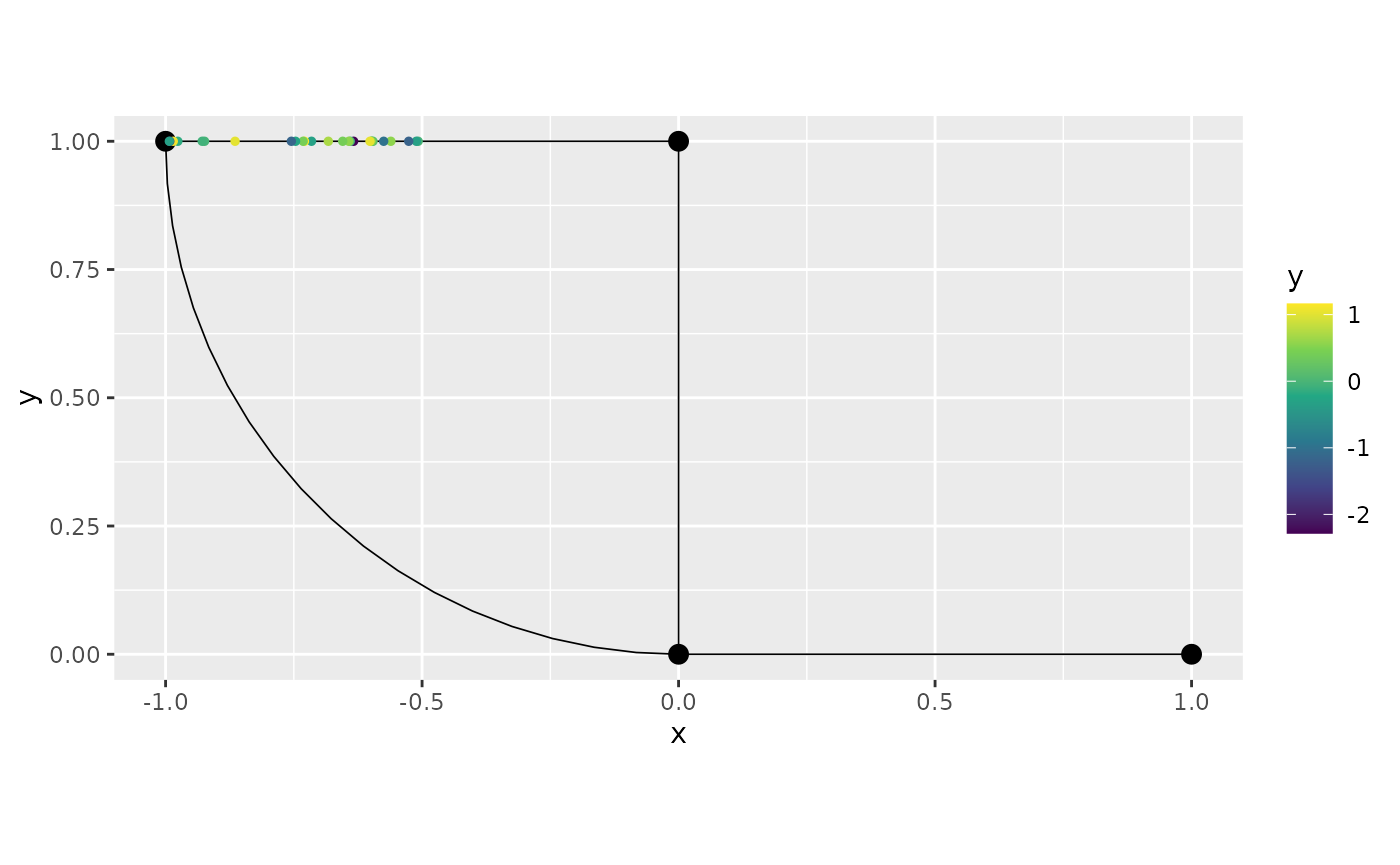
The behavior with NA variables is exactly the same as
with the select() method. For example, we can remove the
rows that contain NA variables by setting
drop_na to TRUE:
graph$filter(y > 1, .drop_na = TRUE)## # A tibble: 30 × 10
## y y2 y3 y4 .edge_number .distance_on_edge .group .loc_idx
## <dbl> <dbl> <dbl> <dbl> <dbl> <dbl> <chr> <int>
## 1 1.34 3.83 1.80 0.974 1 0.212 1 10
## 2 1.18 3.24 1.38 0.923 1 0.647 1 29
## 3 1.43 4.19 2.05 0.990 1 0.687 1 33
## 4 1.77 5.85 3.12 0.981 1 0.898 1 46
## 5 2.21 9.08 4.87 0.805 2 0.258 1 61
## 6 1.00 2.72 1.00 0.841 2 0.316 1 63
## 7 2.31 10.1 5.33 0.740 2 0.339 1 67
## 8 2.08 7.97 4.31 0.875 2 0.390 1 69
## 9 1.87 6.48 3.49 0.956 2 0.407 1 71
## 10 1.44 4.23 2.08 0.992 2 0.455 1 75
## # ℹ 20 more rows
## # ℹ 2 more variables: .coord_x <dbl>, .coord_y <dbl>To conclude, we can also use the filter() function on
top of the result of the get_data() method:
Let us plot:
graph$plot(data = "y", newdata = filtered_data2)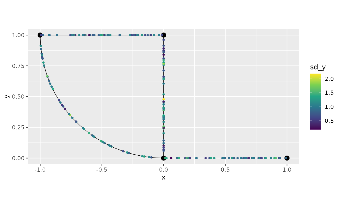
mutate
The mutate verb creates new columns, or modify existing
columns, as functions of the existing columns. Let us create a new
column, new_y, obtained as the sum of y and
y2:
graph$mutate(new_y = y+y2)## # A tibble: 200 × 11
## y y2 y3 y4 .edge_number .distance_on_edge .group .loc_idx
## <dbl> <dbl> <dbl> <dbl> <dbl> <dbl> <chr> <int>
## 1 NA NA NA NA 1 0.0134 1 1
## 2 2.09 NA 4.36 0.870 1 0.0233 1 2
## 3 1.68 5.38 NA 0.994 1 0.0618 1 3
## 4 -0.528 0.590 0.279 -0.504 1 0.108 1 4
## 5 -0.180 0.836 0.0322 -0.179 1 0.126 1 5
## 6 -0.462 0.630 0.213 -0.445 1 0.177 1 6
## 7 -1.52 0.219 2.31 -0.999 1 0.186 1 7
## 8 -0.655 0.520 0.428 -0.609 1 0.202 1 8
## 9 -0.636 0.530 0.404 -0.594 1 0.206 1 9
## 10 1.34 3.83 1.80 0.974 1 0.212 1 10
## # ℹ 190 more rows
## # ℹ 3 more variables: .coord_x <dbl>, .coord_y <dbl>, new_y <dbl>The behavior with NA data is the same as for the
filter() and select() methods. For example, if
we want to keep all the data, we can set .drop_all_na to
`FALSE:
graph$mutate(new_y = y+y2, .drop_all_na=FALSE)## # A tibble: 200 × 11
## y y2 y3 y4 .edge_number .distance_on_edge .group .loc_idx
## <dbl> <dbl> <dbl> <dbl> <dbl> <dbl> <chr> <int>
## 1 NA NA NA NA 1 0.0134 1 1
## 2 2.09 NA 4.36 0.870 1 0.0233 1 2
## 3 1.68 5.38 NA 0.994 1 0.0618 1 3
## 4 -0.528 0.590 0.279 -0.504 1 0.108 1 4
## 5 -0.180 0.836 0.0322 -0.179 1 0.126 1 5
## 6 -0.462 0.630 0.213 -0.445 1 0.177 1 6
## 7 -1.52 0.219 2.31 -0.999 1 0.186 1 7
## 8 -0.655 0.520 0.428 -0.609 1 0.202 1 8
## 9 -0.636 0.530 0.404 -0.594 1 0.206 1 9
## 10 1.34 3.83 1.80 0.974 1 0.212 1 10
## # ℹ 190 more rows
## # ℹ 3 more variables: .coord_x <dbl>, .coord_y <dbl>, new_y <dbl>Let us modify the variable y3 and at the same time
remove all the NA:
graph$mutate(y3 = ifelse(y>1,1,-1), .drop_na = TRUE)## # A tibble: 197 × 10
## y y2 y3 y4 .edge_number .distance_on_edge .group .loc_idx
## <dbl> <dbl> <dbl> <dbl> <dbl> <dbl> <chr> <int>
## 1 -0.528 0.590 -1 -0.504 1 0.108 1 4
## 2 -0.180 0.836 -1 -0.179 1 0.126 1 5
## 3 -0.462 0.630 -1 -0.445 1 0.177 1 6
## 4 -1.52 0.219 -1 -0.999 1 0.186 1 7
## 5 -0.655 0.520 -1 -0.609 1 0.202 1 8
## 6 -0.636 0.530 -1 -0.594 1 0.206 1 9
## 7 1.34 3.83 1 0.974 1 0.212 1 10
## 8 -0.620 0.538 -1 -0.581 1 0.266 1 11
## 9 -0.100 0.905 -1 -0.100 1 0.267 1 12
## 10 -0.324 0.723 -1 -0.319 1 0.340 1 13
## # ℹ 187 more rows
## # ℹ 2 more variables: .coord_x <dbl>, .coord_y <dbl>Finally, we can also apply the mutate() function the
result of the get_data() method, and also pipe it to the
plot() method (we are also changing the scale to
discrete):
library(ggplot2)

graph$get_data() %>% mutate(new_y = y+y2,
                        y3=as.factor(ifelse(y>1,1,-1))) %>%
                        graph$plot(data = "y3") +
                        scale_colour_discrete()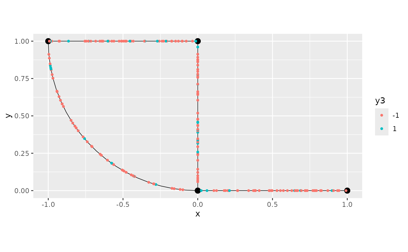
summarise
The summarise verb creates summaries of selected columns
based on groupings. For metric graphs, the groups always include the
edge number (.edge_number) and relative distance on edge
(.distance_on_edge). By using the argument
.include_graph_groups, the internal metric graph group
variable, namely .group, will also be added to the
summarise() group. Finally, additional groups can be passed
by the .groups argument.
To illustrate, we will use the data.frame from the group
example:
graph$add_observations(data = df_data_repl,
                normalized = TRUE,
                clear_obs = TRUE,
                group = "repl")
## Adding observations...## Assuming the observations are normalized by the length of the edge.We can see the data:
graph$get_data()## # A tibble: 1,000 × 8
## y repl .edge_number .distance_on_edge .group .loc_idx .coord_x .coord_y
## <dbl> <int> <dbl> <dbl> <chr> <int> <dbl> <dbl>
## 1 1.50 1 1 0.0134 1 1 0.0134 0
## 2 -1.79 1 1 0.0233 1 2 0.0233 0
## 3 0.488 1 1 0.0618 1 3 0.0618 0
## 4 -0.385 1 1 0.108 1 4 0.108 0
## 5 0.905 1 1 0.126 1 5 0.126 0
## 6 -0.145 1 1 0.177 1 6 0.177 0
## 7 2.00 1 1 0.186 1 7 0.186 0
## 8 -1.16 1 1 0.202 1 8 0.202 0
## 9 0.879 1 1 0.206 1 9 0.206 0
## 10 -0.816 1 1 0.212 1 10 0.212 0
## # ℹ 990 more rowsLet us summarise the data by obtaining the mean of
y at each location across all groups:
graph$summarise(mean_y = mean(y))## # A tibble: 200 × 6
## .edge_number .distance_on_edge .coord_x .coord_y mean_y .group
## <dbl> <dbl> <dbl> <dbl> <dbl> <dbl>
## 1 1 0.0134 0.0134 0 0.578 1
## 2 1 0.0233 0.0233 0 0.407 1
## 3 1 0.0618 0.0618 0 0.638 1
## 4 1 0.108 0.108 0 -0.327 1
## 5 1 0.126 0.126 0 -0.942 1
## 6 1 0.177 0.177 0 -0.156 1
## 7 1 0.186 0.186 0 0.0925 1
## 8 1 0.202 0.202 0 -0.0548 1
## 9 1 0.206 0.206 0 0.345 1
## 10 1 0.212 0.212 0 -0.546 1
## # ℹ 190 more rowsLet us now obtain the standard deviation of y at each
location and plot it:
drop_na
The drop_na verb removes rows that contain
NA for the selected columns. To illustrate, let us add the
df_tidy back to the metric graph, replacing the existing
dataset:
graph$add_observations(data = df_tidy, clear_obs=TRUE, normalized=TRUE)## Adding observations...## Assuming the observations are normalized by the length of the edge.Now, let us take a look at this dataset:
graph$get_data(drop_all_na = FALSE)## # A tibble: 200 × 10
## y y2 y3 y4 .edge_number .distance_on_edge .group .loc_idx
## <dbl> <dbl> <dbl> <dbl> <dbl> <dbl> <chr> <int>
## 1 NA NA NA NA 1 0.0134 1 1
## 2 2.09 NA 4.36 0.870 1 0.0233 1 2
## 3 1.68 5.38 NA 0.994 1 0.0618 1 3
## 4 -0.528 0.590 0.279 -0.504 1 0.108 1 4
## 5 -0.180 0.836 0.0322 -0.179 1 0.126 1 5
## 6 -0.462 0.630 0.213 -0.445 1 0.177 1 6
## 7 -1.52 0.219 2.31 -0.999 1 0.186 1 7
## 8 -0.655 0.520 0.428 -0.609 1 0.202 1 8
## 9 -0.636 0.530 0.404 -0.594 1 0.206 1 9
## 10 1.34 3.83 1.80 0.974 1 0.212 1 10
## # ℹ 190 more rows
## # ℹ 2 more variables: .coord_x <dbl>, .coord_y <dbl>For example, let us remove the rows such that y3 is
NA, we simply apply the drop_na() method
passing the column y3:
graph$drop_na(y3)## # A tibble: 198 × 10
## y y2 y3 y4 .edge_number .distance_on_edge .group .loc_idx
## <dbl> <dbl> <dbl> <dbl> <dbl> <dbl> <chr> <int>
## 1 2.09 NA 4.36 0.870 1 0.0233 1 2
## 2 -0.528 0.590 0.279 -0.504 1 0.108 1 4
## 3 -0.180 0.836 0.0322 -0.179 1 0.126 1 5
## 4 -0.462 0.630 0.213 -0.445 1 0.177 1 6
## 5 -1.52 0.219 2.31 -0.999 1 0.186 1 7
## 6 -0.655 0.520 0.428 -0.609 1 0.202 1 8
## 7 -0.636 0.530 0.404 -0.594 1 0.206 1 9
## 8 1.34 3.83 1.80 0.974 1 0.212 1 10
## 9 -0.620 0.538 0.385 -0.581 1 0.266 1 11
## 10 -0.100 0.905 0.0100 -0.100 1 0.267 1 12
## # ℹ 188 more rows
## # ℹ 2 more variables: .coord_x <dbl>, .coord_y <dbl>We can also remove the rows such that either y2 or
y3 is NA:
graph$drop_na(y2, y3)## # A tibble: 197 × 10
## y y2 y3 y4 .edge_number .distance_on_edge .group .loc_idx
## <dbl> <dbl> <dbl> <dbl> <dbl> <dbl> <chr> <int>
## 1 -0.528 0.590 0.279 -0.504 1 0.108 1 4
## 2 -0.180 0.836 0.0322 -0.179 1 0.126 1 5
## 3 -0.462 0.630 0.213 -0.445 1 0.177 1 6
## 4 -1.52 0.219 2.31 -0.999 1 0.186 1 7
## 5 -0.655 0.520 0.428 -0.609 1 0.202 1 8
## 6 -0.636 0.530 0.404 -0.594 1 0.206 1 9
## 7 1.34 3.83 1.80 0.974 1 0.212 1 10
## 8 -0.620 0.538 0.385 -0.581 1 0.266 1 11
## 9 -0.100 0.905 0.0100 -0.100 1 0.267 1 12
## 10 -0.324 0.723 0.105 -0.319 1 0.340 1 13
## # ℹ 187 more rows
## # ℹ 2 more variables: .coord_x <dbl>, .coord_y <dbl>If we simply run the drop_na() method, this is
equivalent to run the get_data() method with the argument
drop_na set to TRUE:
identical(graph$drop_na(), graph$get_data(drop_na=TRUE))## [1] FALSEFinally, we can also directly apply the drop_na()
function to the result of the get_data() method:
## # A tibble: 198 × 10
##         y     y2     y3     y4 .edge_number .distance_on_edge .group .loc_idx
##     <dbl>  <dbl>  <dbl>  <dbl>        <dbl>             <dbl> <chr>     <int>
##  1  2.09  NA     4.36    0.870            1            0.0233 1             2
##  2 -0.528  0.590 0.279  -0.504            1            0.108  1             4
##  3 -0.180  0.836 0.0322 -0.179            1            0.126  1             5
##  4 -0.462  0.630 0.213  -0.445            1            0.177  1             6
##  5 -1.52   0.219 2.31   -0.999            1            0.186  1             7
##  6 -0.655  0.520 0.428  -0.609            1            0.202  1             8
##  7 -0.636  0.530 0.404  -0.594            1            0.206  1             9
##  8  1.34   3.83  1.80    0.974            1            0.212  1            10
##  9 -0.620  0.538 0.385  -0.581            1            0.266  1            11
## 10 -0.100  0.905 0.0100 -0.100            1            0.267  1            12
## # ℹ 188 more rows
## # ℹ 2 more variables: .coord_x <dbl>, .coord_y <dbl>Combining multiple verbs
The resulting data from applying the previous verbs are safe in the sense that they are friendly to the metric graph environment. Thus, the result after applying one verb can be used as input of any of the remaining verbs.
For this example we will consider the df_data_repl
dataset. Let us add to the graph (replacing the existing data):
graph$add_observations(data = df_data_repl,
                        normalized = TRUE,
                        clear_obs = TRUE,
                        group = "repl")
## Adding observations...## Assuming the observations are normalized by the length of the edge.
graph$get_data(drop_all_na = FALSE)## # A tibble: 1,000 × 8
## y repl .edge_number .distance_on_edge .group .loc_idx .coord_x .coord_y
## <dbl> <int> <dbl> <dbl> <chr> <int> <dbl> <dbl>
## 1 1.50 1 1 0.0134 1 1 0.0134 0
## 2 -1.79 1 1 0.0233 1 2 0.0233 0
## 3 0.488 1 1 0.0618 1 3 0.0618 0
## 4 -0.385 1 1 0.108 1 4 0.108 0
## 5 0.905 1 1 0.126 1 5 0.126 0
## 6 -0.145 1 1 0.177 1 6 0.177 0
## 7 2.00 1 1 0.186 1 7 0.186 0
## 8 -1.16 1 1 0.202 1 8 0.202 0
## 9 0.879 1 1 0.206 1 9 0.206 0
## 10 -0.816 1 1 0.212 1 10 0.212 0
## # ℹ 990 more rowsWe will now create a new variable new_y which is the
exponential of y, then filter the data to be on edges
1 and 2, summarise to get the means of
new_y at all positions (across the different groups, from
the _.group variable) and plot it:
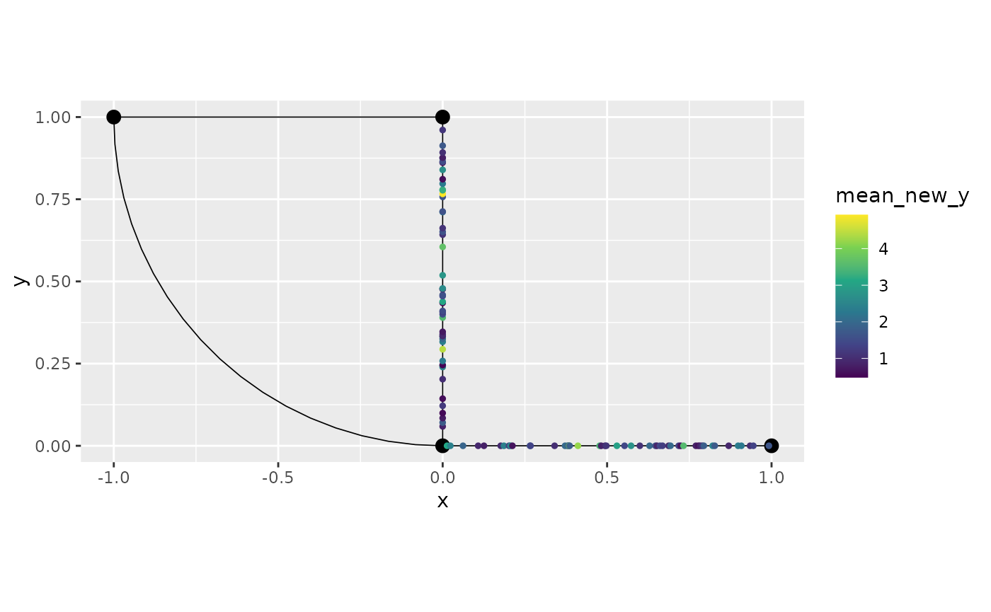
graph$mutate(new_y = exp(y)) %>% filter(`.edge_number` %in% c(1,2)) %>%
            summarise(mean_new_y = mean(new_y)) %>%
            graph$plot(data = "mean_new_y")
Replacing the data in the metric graph by manipulated data
Let us suppose we want to replace the internal data by the data
obtained from these manipulations. This is very simple, all we need to
do is to pass the resulting data to the data argument from
the add_observations() method. It is important to note that
if the input is the result of those verbs, mutate,
select, filter, summarise or
drop_na, or any combination of them, then there is no need
to set any of the other arguments of the add_observations()
method, one should simply supply the data argument with
such dataset. For example, let us consider the dataset from the previous
section. We will replace the data, so we will set clear_obs
to TRUE:
graph$add_observations(data = graph$mutate(new_y = exp(y)) %>%
                        filter(`.edge_number` %in% c(1,2)) %>%
                                summarise(mean_new_y = mean(new_y)),
                                clear_obs = TRUE)
## Adding observations...## Assuming the observations are NOT normalized by the length of the edge.We can now observe the result:
graph$get_data()## # A tibble: 100 × 7
## .coord_x .coord_y mean_new_y .edge_number .distance_on_edge .group .loc_idx
## <dbl> <dbl> <dbl> <dbl> <dbl> <chr> <int>
## 1 0.0134 0 3.15 1 0.0134 1 1
## 2 0.0233 0 2.43 1 0.0233 1 2
## 3 0.0618 0 1.92 1 0.0618 1 3
## 4 0.108 0 0.931 1 0.108 1 4
## 5 0.126 0 0.814 1 0.126 1 5
## 6 0.177 0 0.968 1 0.177 1 6
## 7 0.186 0 2.40 1 0.186 1 7
## 8 0.202 0 1.24 1 0.202 1 8
## 9 0.206 0 2.60 1 0.206 1 9
## 10 0.212 0 0.643 1 0.212 1 10
## # ℹ 90 more rowsWe can also save it to a separate variable and use as input:
df_temp <- graph$mutate(even_newer_y = mean_new_y^2)
graph$add_observations(data = df_temp, clear_obs = TRUE)
## Adding observations...## Assuming the observations are NOT normalized by the length of the edge.We can check that it was properly added:
graph$get_data()## # A tibble: 100 × 8
## .coord_x .coord_y mean_new_y even_newer_y .edge_number .distance_on_edge
## <dbl> <dbl> <dbl> <dbl> <dbl> <dbl>
## 1 0.0134 0 3.15 9.90 1 0.0134
## 2 0.0233 0 2.43 5.89 1 0.0233
## 3 0.0618 0 1.92 3.69 1 0.0618
## 4 0.108 0 0.931 0.867 1 0.108
## 5 0.126 0 0.814 0.663 1 0.126
## 6 0.177 0 0.968 0.937 1 0.177
## 7 0.186 0 2.40 5.76 1 0.186
## 8 0.202 0 1.24 1.53 1 0.202
## 9 0.206 0 2.60 6.73 1 0.206
## 10 0.212 0 0.643 0.413 1 0.212
## # ℹ 90 more rows
## # ℹ 2 more variables: .group <chr>, .loc_idx <int>Edge Weights Manipulation in Metric Graphs
We will demonstrate edge weights manipulation using various
tidyverse-style verbs, including select,
mutate, filter, summarise, and
drop_na. We will also introduce some NA values
for illustration.
Adding Edge Weights to the Metric Graph
We begin by creating a dataset of edge weights and adding it to the metric graph:
set.seed(123)

# Generate edge weight data
edge_weights_df <- data.frame(
  weight = runif(graph$nE),
  weight2 = rnorm(graph$nE),
  weight3 = runif(graph$nE) * 100
)

# Introduce some NA values
edge_weights_df$weight[1] <- NA
edge_weights_df$weight2[2] <- NA
edge_weights_df$weight3[3] <- NA

# Set edge weights in the metric graph
graph$set_edge_weights(weights = edge_weights_df)

# Display the edge weights
graph$get_edge_weights()
## # A tibble: 4 × 4
## weight weight2 weight3 .weights
## <dbl> <dbl> <dbl> <dbl>
## 1 NA 1.56 67.8 1
## 2 0.788 NA 57.3 1
## 3 0.409 0.129 NA 1
## 4 0.883 1.72 90.0 1Selecting Specific Edge Weight Columns
The select_weights() method allows us to choose specific
columns from the edge weight dataset. Let’s select weight
and weight2, while preserving all rows, even if they
contain NA:
graph$select_weights(weight, weight2, .drop_all_na = FALSE)## # A tibble: 4 × 2
## weight weight2
## <dbl> <dbl>
## 1 NA 1.56
## 2 0.788 NA
## 3 0.409 0.129
## 4 0.883 1.72Filtering Edge Weights
We can filter rows based on conditions. For example, let’s filter
rows where weight > 0.5 and remove rows containing
NA values:
graph$filter_weights(weight > 0.5, .drop_na = TRUE)## # A tibble: 1 × 4
## weight weight2 weight3 .weights
## <dbl> <dbl> <dbl> <dbl>
## 1 0.883 1.72 90.0 1We can also filter edge weights using standard tidyverse functions:
Creating New Columns Using mutate_weights()
We will now create a new column weight_log, which is the
logarithm of weight + 1:
graph$mutate_weights(weight_log = log(weight + 1))## # A tibble: 4 × 5
## weight weight2 weight3 .weights weight_log
## <dbl> <dbl> <dbl> <dbl> <dbl>
## 1 NA 1.56 67.8 1 NA
## 2 0.788 NA 57.3 1 0.581
## 3 0.409 0.129 NA 1 0.343
## 4 0.883 1.72 90.0 1 0.633We can plot the result after applying the mutation. To this end, we
first set the new edges as the result from mutate_weights,
then we plot:
graph$set_edge_weights(weights = graph$mutate_weights(weight_log = log(weight + 1)))
graph$plot(edge_weight = "weight_log")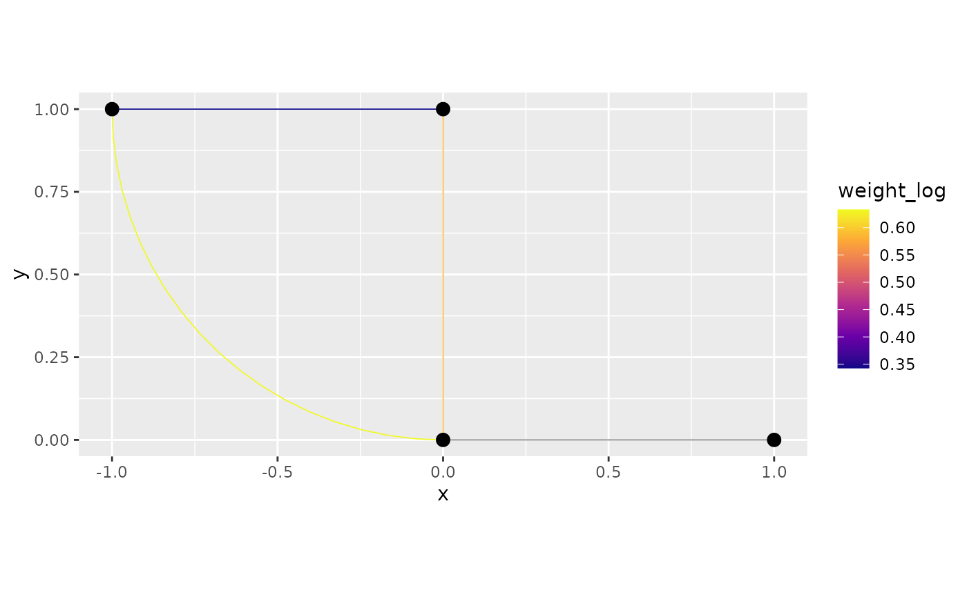
Summarising Edge Weights
We can summarise edge weights by calculating the mean of
weight and weight2 for all edges:
graph$summarise_weights(mean_weight = mean(weight, na.rm = TRUE),
                        mean_weight2 = mean(weight2, na.rm = TRUE))
## # A tibble: 1 × 2
## mean_weight mean_weight2
## <dbl> <dbl>
## 1 0.693 1.13If we want to group by edge numbers or other columns, we can use the
.groups argument:
graph$summarise_weights(mean_weight = mean(weight, na.rm = TRUE),
                        mean_weight2 = mean(weight2, na.rm = TRUE),
                        .groups = ".weights")
## # A tibble: 1 × 3
## .weights mean_weight mean_weight2
## <dbl> <dbl> <dbl>
## 1 1 0.693 1.13Removing Rows with NA Values
To remove rows that contain NA values for the
weight and weight2 columns, we use the
drop_na_weights() method:
graph$drop_na_weights(weight, weight2)## # A tibble: 2 × 5
## weight weight2 weight3 .weights weight_log
## <dbl> <dbl> <dbl> <dbl> <dbl>
## 1 0.409 0.129 NA 1 0.343
## 2 0.883 1.72 90.0 1 0.633We can also directly apply drop_na() to the result of
get_edge_weights():
## # A tibble: 2 × 5
##   weight weight2 weight3 .weights weight_log
##    <dbl>   <dbl>   <dbl>    <dbl>      <dbl>
## 1  0.409   0.129    NA          1      0.343
## 2 0.883 1.72 90.0 1 0.633Combining Multiple Verbs
Finally, let us combine multiple verbs to manipulate the edge weights. We will mutate the weights, filter for certain conditions, and summarise them:
graph$mutate_weights(new_weight = weight * 10) %>%
       filter(weight > 0.2) %>%
       summarise(mean_new_weight = mean(new_weight, na.rm = TRUE))
## # A tibble: 1 × 1
## mean_new_weight
## <dbl>
## 1 6.93