Solving PDEs on metric graphs

David Bolin

Created: 2025-03-10. Last modified: 2025-03-21.

Introduction

In this vignette we will introduce how to solve some basic PDEs on metric graphs.

For details on the construction of metric graphs, see Working with metric graphs

For further details on data manipulation on metric graphs, see Data manipulation on metric graphs

Constructing the graph and the mesh

We begin by loading the rSPDE and MetricGraph packages:

  library(rSPDE)
  library(MetricGraph)

As an example, we consider the logo graph

  graph <- metric_graph$new(perform_merges = TRUE, 
                            tolerance = list(edge_edge = 1e-3, 
                                             vertex_vertex = 1e-3, 
                                             edge_vertex = 1e-3))
  graph$plot()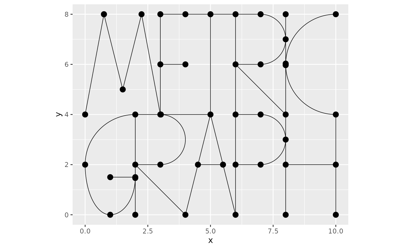

To construct a FEM approximation of a PDE on this graph, we first must construct a mesh on the graph.

  graph$build_mesh(h = 0.2)
  graph$plot(mesh=TRUE)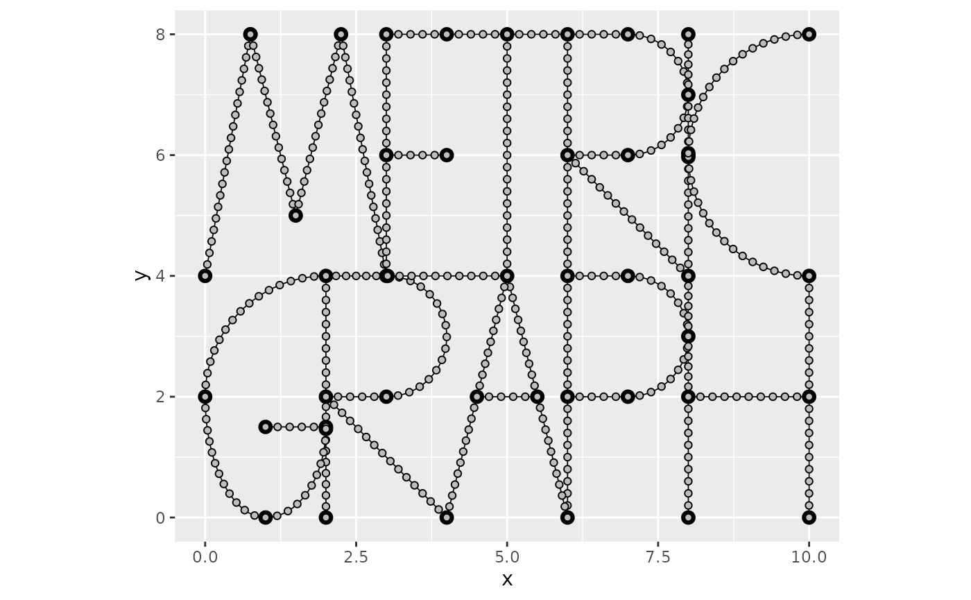

In the command build_mesh, the argument h decides the largest spacing between nodes in the mesh.

Example with the Helmoltz equation

As a simple first problem, let us consider solving the Helmholtz equation $$(\kappa^2 - \Delta) u = f,$$ where the operator is equipped with Kirchhoff vertex conditions and we assume that $\kappa = 1$. Discretizing the problem through a Galerkin FEM method yields a solution $u_h(s) = \sum_{i=1}^n u_i \varphi_i(s)$ where $\{\varphi_i\}$ are the hat functions induced by the mesh and $\mathbf{u} = (u_1,\ldots, u_n)$ are the weights, which solve $$(\kappa^2 \mathbf{C} + \mathbf{G}) \mathbf{u} = \mathbf{f}.$$ Here $\mathbf{C}$ is the mass matrix with elements $C_{ij} = (\varphi_i, \varphi_j)_{L_2(\Gamma)}$, $\mathbf{G}$ is the stiffness matrix with elements $G_{ij} = (\nabla \varphi_i, \nabla \varphi_j)_{L_2(\Gamma)}$, and $f_i = (\varphi_i, f)_{L_2(\Gamma)}$. The mass and stiffness matrices can be computed as follows

  graph$compute_fem()
  G <- graph$mesh$G
  C <- graph$mesh$C

Suppose that $f(s) = x^2 - y^2$, where $(x,y)$ are the Euclidean coordinates of the location $s$ on the graph. We approximate this function as being piecewise linear on the mesh and compute $\mathbf{f} = \mathbf{C}\bar{f}$, where $\bar{f}$ is a vector with $f$ evaluated at the mesh nodes

x <- graph$mesh$V[, 1]
y <- graph$mesh$V[, 2]
fbar <- x^2 - y^2
C <- graph$mesh$C
f <- C%*%fbar
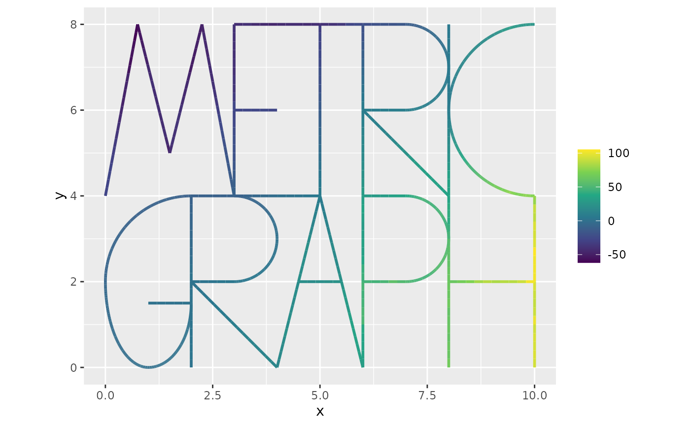
graph$plot_function(fbar, vertex_size = 0)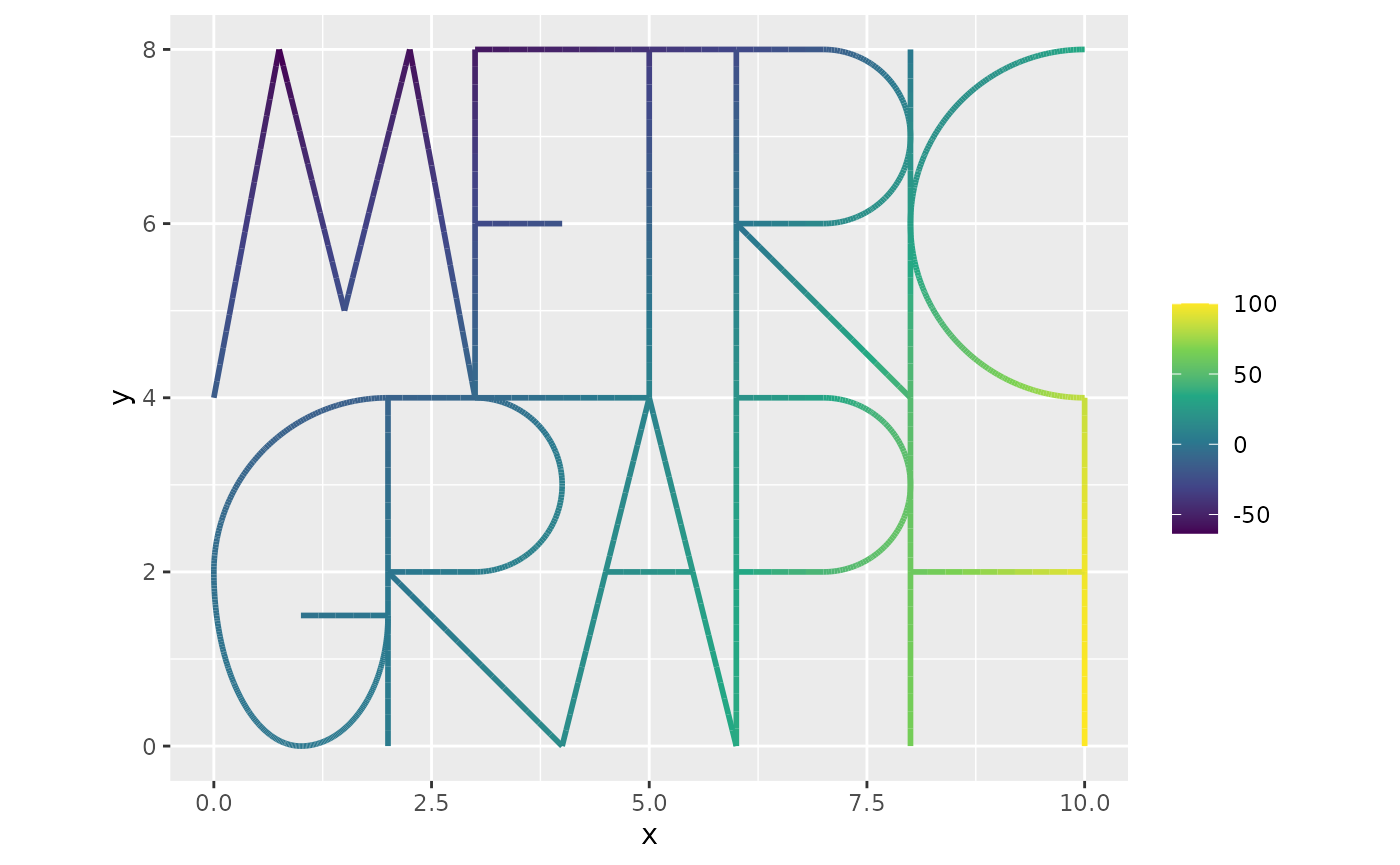

We now solve the system as

kappa <- 1
L <- kappa^2*C + G
u <- solve(L,f)
graph$plot_function(u,vertex_size=0)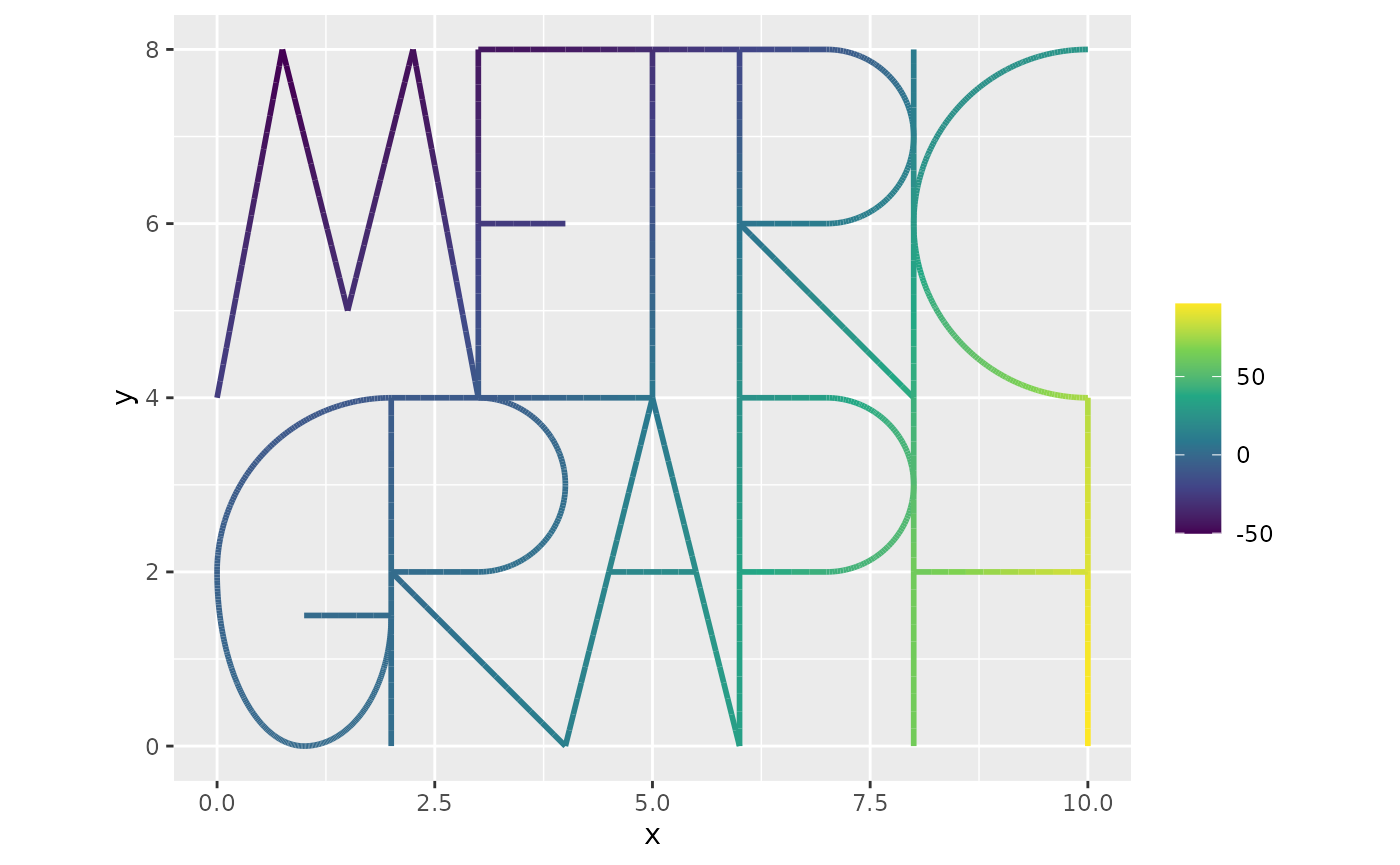

Example with a Poisson equation

Let us now consider the Poisson equation $$-\Delta u = f,$$ where the operator is equipped with Kirchhoff vertex conditions at the vertices of degree $d\geq 2$ and homogeneous Dirichlet vertex conditions at the vertices of degree $d=1$ (to guarantee a unique solution). Again using a Galerkin FEM method yields a solution $u_h(s) = \sum_{i=1}^n u_i \varphi_i(s)$ where $\{\varphi_i\}$ are the hat functions induced by the mesh and $\mathbf{u} = (u_1,\ldots, u_n)$ are the weights, which now solve $$\mathbf{G} \mathbf{u} = \mathbf{f}.$$ The difference is now that we must handle the Dirichlet conditions. By default, the stiffness matrix is computed assuming Kirchhoff vertex conditions at all nodes. Go obtain the matrix corresponding to Dirichlet vertex conditions, we simply have to remove the rows and columns corresponding to the degree 1 vertices:

  n.mesh <- dim(graph$mesh$V)[1]
  ind <- setdiff(1:n.mesh, which(graph$get_degrees()==1))
  Gd <- G[ind,ind]

Suppose that $f(s) = 1(x > 4)$, where $(x,y)$ are the Euclidean coordinates of the location $s$ on the graph. We again approximate this function as being piecewise linear on the mesh and compute $\mathbf{f} = \mathbf{C}\bar{f}$, where $\mathbf{C}$ is the mass matrix with elements $C_{ij} = (\varphi_i, \varphi_j)_{L_2(\Gamma)}$ and $\bar{f}$ is a vector with $f$ evaluated at the mesh nodes

fbar <- x> 4
f <- C%*%fbar
graph$plot_function(fbar, vertex_size = 0)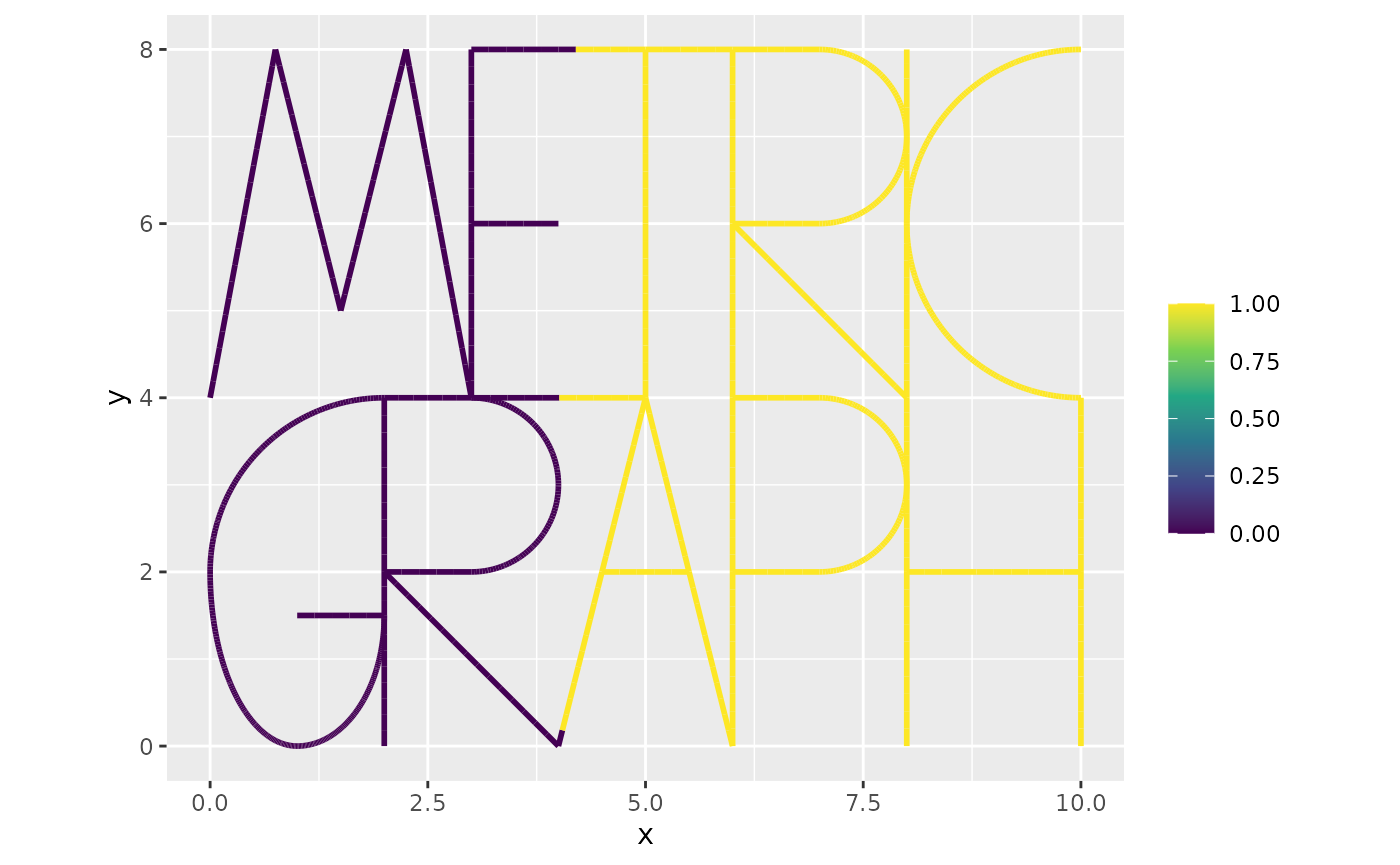

We now solve the system as

f.int <- f[ind]           #Get the load vector at the internal nodes
u.int <- solve(Gd,f.int)  #solve for u at the internal nodes
u <- rep(0, n.mesh)
u[ind] <- u.int           #add the solution to the internal nodes
graph$plot_function(u,vertex_size=0)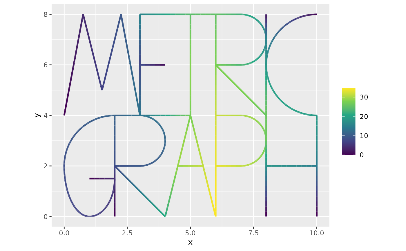

A problem with a random diffusion coefficient

As another example, let us consider the problem $$(\kappa^2 - \nabla\cdot(e^u\nabla)) u = f,$$ where $u$ is a Gaussian process. The only difference to the first example is that we now need to evaluate a stiffness matrix with elements $$G_{ij}(u) = (e^u \nabla \varphi_i, \nabla \varphi_j)_{L_2(\Gamma)}$$ By assuming that $e^u$ is piecewise linear on the mesh, we can write this matrix as $$\mathbf{G}(u) = \frac12(\mathbf{D}(u)\mathbf{G} + \mathbf{G}\mathbf{D}(u))$$ where $\mathbf{D}(u)$ is a diagonal matrix with the values of $e^u$ at the mesh nodes on the diagonal.

Let us now simulate a Gaussian Whittle–Matérn field $u$ at the mesh nodes.

u <- sample_spde(range = 4, sigma = 0.3, alpha = 1, graph = graph, type = "mesh")
graph$plot_function(X = exp(u), vertex_size = 0)

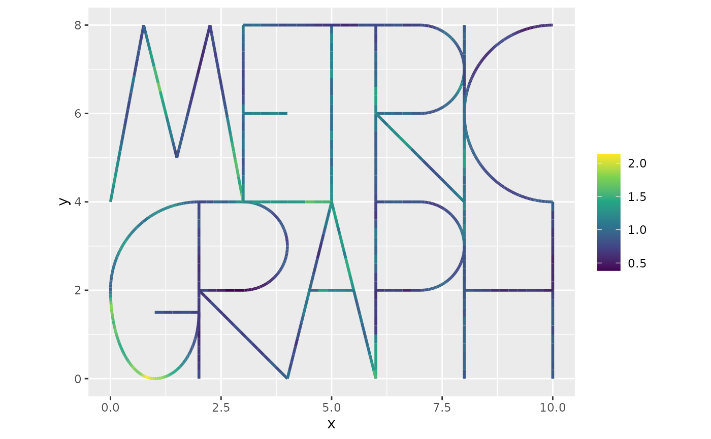
We can now build the matrix $\mathbf{G}(u)$:

Du <- Diagonal(n.mesh, exp(u))
Gu <- (G%*%Du + Du%*%G)/2

Let us use the same right hand side as in the first example and solve the PDE with $\kappa = 1$:

fbar <- x^2 - y^2
f <- C%*%fbar
kappa <- 1
L <- kappa^2*C + Gu
u <- solve(L,f)
graph$plot_function(u,vertex_size=0)

Solving a fractional-order PDE using rSPDE

Finally, let us consider solving a fractional-order version of the PDE in the previous example: $$(\kappa^2 - \nabla\cdot(e^u\nabla))^{\beta} u = f,$$

To solve this, we can use the rSPDE package, to obtain a rational approximation of the fractional power. Specifically, we use the operator-based approach by Bolin and Kirchner (2020), which results in an approximation of the original PDE which is of the form $P_l u(s) = P_r f(s)$, where $P_l$ and $P_r$ are non-fractional operators defined in terms of polynomials $p_l$ and $p_r$. The order of $p_r$ is given by $m$ and the order of $p_l$ is $m + m_{\beta}$ where $m_{\beta}$ is the integer part of $\beta$ if $\beta>1$ and $m_{\beta} = 1$ otherwise.

Having already computed the FEM approximation of the operator $L = \kappa^2 - \nabla\cdot(e^u\nabla)$, we can use the function fractional.operators to define the rational approximation. For this we just have to provide the operator, mass matrix, $\beta$, the order of the rational approximation, and a scale factor which is a lower bound for the eigenvalues of $L$. In this case, a lower bound is given by $\kappa^2$.

library(rSPDE)
beta <- 1.5
op <- fractional.operators(L, beta, C, scale.factor = kappa^2, m = 1)

We can now solve the problem as follows

u <- Pl.solve(op, Pr.mult(op, f))
graph$plot_function(u,vertex_size=0)

References

Bolin, David, and Kristin Kirchner. 2020. “The Rational SPDE Approach for Gaussian Random Fields with General Smoothness.” Journal of Computational and Graphical Statistics 29 (2): 274–85.