Connected components of metric graph

graph_components is deprecated. metric_graph now handles disconnected graphs directly: construct it with check_connected = FALSE, then use mg$get_components() to obtain a list of per-component metric_graph objects, mg$which_component(XY) to route spatial points, and mg$plot(components = TRUE) to colour the components. Distance methods (compute_geodist, compute_resdist, compute_laplacian) and SPDE machinery (spde_precision, sample_spde, graph_lme, ...) all work on disconnected metric_graph objects natively — precision matrices come out block-diagonal by construction.

Value

Object of R6Class for creating metric graph components.

Details

A list of metric_graph objects (representing the different connected components in the full graph) created from vertex and edge matrices, or from an sp::SpatialLines object where each line is representing and edge. For more details, see the vignette: vignette("metric_graph", package = "MetricGraph")

Public fields

graphs: List of the graphs representing the connected components.
n: The number of graphs.
sizes: Number of vertices for each of the graphs.
lengths: Total edge lengths for each of the graphs.
nE_total: Total number of edges across all components.
edge_offsets: Integer vector of length n giving the cumulative number of edges in components before each one. The global edge number of local edge e in component k is edge_offsets[k] + e. Create metric graphs for connected components

Methods

`graph_components$new()`

Usage

graph_components$new(
  edges = NULL,
  V = NULL,
  E = NULL,
  by_length = TRUE,
  edge_weights = NULL,
  ...,
  lines = deprecated()
)

Arguments

edges: A list containing coordinates as m x 2 matrices (that is, of matrix type) or m x 2 data frames (data.frame type) of sequence of points connected by straightlines. Alternatively, you can also prove an object of type SpatialLinesDataFrame or SpatialLines (from sp package) or MULTILINESTRING (from sf package).
V: n x 2 matrix with Euclidean coordinates of the n vertices.
E: m x 2 matrix where each row represents an edge.
by_length: Sort the components by total edge length? If FALSE, the components are sorted by the number of vertices.
edge_weights: Either a number, a numerical vector with length given by the number of edges, providing the edge weights, or a data.frame with the number of rows being equal to the number of edges, where
...: Additional arguments used when specifying the graphs
lines: Use edges instead.
vertex_unit: The unit in which the vertices are specified. The options are 'degree' (the great circle distance in km), 'km', 'm' and 'miles'. The default is NULL, which means no unit. However, if you set length_unit, you need to set vertex_unit.
length_unit: The unit in which the lengths will be computed. The options are 'km', 'm' and 'miles'. The default is vertex_unit. Observe that if vertex_unit is NULL, length_unit can only be NULL. If vertex_unit is 'degree', then the default value for length_unit is 'km'.
longlat: If TRUE, then it is assumed that the coordinates are given. in Longitude/Latitude and that distances should be computed in meters. It takes precedence over vertex_unit and length_unit, and is equivalent to vertex_unit = 'degree' and length_unit = 'm'.
tolerance: Vertices that are closer than this number are merged when constructing the graph (default = 1e-10). If longlat = TRUE, the tolerance is given in km.

Returns

A graph_components object.

`graph_components$edge_to_component()`

Map global edge numbers to component indices. Each edge in the disconnected graph has a unique global edge number; this method returns the component each edge belongs to.

Usage

graph_components$edge_to_component(edge_number)

Arguments

edge_number: Integer vector of global edge numbers in 1:self$nE_total.

Returns

Integer vector of component indices, the same length as edge_number.

`graph_components$get_largest()`

Returns the largest component in the graph.

Usage

graph_components$get_largest()

Returns

A metric_graph object.

`graph_components$as_metric_graph()`

Combine all components into a single (disconnected) metric_graph object via fast in-memory stacking. Edges keep their relative order within each component, and the .edge_number of every observation is shifted by the cumulative edge count of preceding components. The resulting graph carries a disconnected = TRUE flag (queryable via metric_graph$is_disconnected()); calling add_observations() on the returned graph is disallowed because the user-facing edge numbering is no longer the per-component one — add observations to the original graph_components and call as_metric_graph() again.

Call this method explicitly before passing to repeated downstream operations (e.g., graph_lme, graph_spde, sample_spde) to amortise the assembly cost across calls.

Usage

graph_components$as_metric_graph()

Returns

A metric_graph object representing the disjoint union of the components, with mesh and FEM matrices block-diagonally stacked when every component has them.

`graph_components$which_component()`

For each spatial point, determine which component it belongs to. The component is the one whose nearest network location is closest in Euclidean distance to the point.

Usage

graph_components$which_component(XY)

Arguments

XY: An n x 2 matrix of spatial coordinates.

Returns

An integer vector of length n with the component index for each point.

`graph_components$add_observations()`

Add observations to the components. Mirrors metric_graph$add_observations. For data_coords = "spatial", each observation is routed to the component whose nearest network location is closest to it. For data_coords = "PtE", the data specifies a global edge_number (in 1:self$nE_total) and the component is inferred automatically from it.

Usage

graph_components$add_observations(
  data = NULL,
  edge_number = "edge_number",
  distance_on_edge = "distance_on_edge",
  coord_x = "coord_x",
  coord_y = "coord_y",
  data_coords = c("PtE", "spatial"),
  group = NULL,
  normalized = FALSE,
  clear_obs = FALSE,
  verbose = 1,
  suppress_warnings = FALSE,
  ...
)

Arguments

data: A data.frame, list, sf object, or SpatialPointsDataFrame with the observations.
edge_number: Name of the (global) edge-number column. Default is "edge_number".
distance_on_edge: Name of the distance-on-edge column. Default is "distance_on_edge".
coord_x: Name of the x-coordinate column. Default is "coord_x".
coord_y: Name of the y-coordinate column. Default is "coord_y".
data_coords: Either "PtE" (the convention is then (edge_number, distance_on_edge) with global edge numbering) or "spatial".
group: Optional grouping variable, see metric_graph$add_observations.
normalized: If TRUE, distances are assumed normalized to (0,1).
clear_obs: If TRUE, all existing observations are cleared first.
verbose: Verbosity level.
suppress_warnings: If TRUE, warnings from the per-component add_observations are suppressed.
...: Additional arguments forwarded to each component's add_observations method.

Returns

No return value. Called for its side effects.

`graph_components$clear_observations()`

Clear observations from all components.

Usage

graph_components$clear_observations()

Returns

No return value. Called for its side effects.

`graph_components$get_data()`

Combine observations from all components. Returns a single data structure with an additional .component column indicating which component each row belongs to.

Usage

graph_components$get_data(
  group = NULL,
  format = c("tibble", "sf", "sp", "list"),
  drop_na = FALSE,
  drop_all_na = TRUE
)

Arguments

group: Optional group filter passed to each component's get_data.
format: One of "tibble", "sf", "sp", "list".
drop_na: See metric_graph$get_data.
drop_all_na: See metric_graph$get_data.

Returns

A combined data object with a .component column.

`graph_components$get_groups()`

Get the unique groups across all components.

Usage

graph_components$get_groups()

Returns

Character vector of unique group identifiers.

`graph_components$get_PtE()`

Get the (edge_number, distance_on_edge) pairs for the observations across all components, using global edge numbering.

Usage

graph_components$get_PtE()

Returns

A matrix with two columns: edge_number, distance_on_edge.

`graph_components$coordinates()`

Convert between graph coordinates (global edge_number, distance_on_edge) and spatial coordinates.

Usage

graph_components$coordinates(PtE = NULL, XY = NULL, normalized = TRUE)

Arguments

PtE: A matrix or vector with two columns/entries: (edge_number, distance_on_edge). Edge numbers are global across components.
XY: An n x 2 matrix of spatial coordinates.
normalized: If TRUE, the distances are normalized to (0,1).

Returns

If PtE is supplied, an n x 2 matrix of spatial coordinates. If XY is supplied, an n x 2 matrix with (edge_number, distance_on_edge) using global edge numbering.

`graph_components$build_mesh()`

Build a mesh on each component.

Usage

graph_components$build_mesh(...)

Arguments

...: Arguments forwarded to metric_graph$build_mesh.

Returns

No return value. Called for its side effects.

`graph_components$compute_fem()`

Compute finite-element matrices on each component that has a mesh.

Usage

graph_components$compute_fem(...)

Arguments

...: Arguments forwarded to metric_graph$compute_fem.

Returns

No return value. Called for its side effects.

`graph_components$compute_geodist()`

Compute geodesic distances per component. The geodesic distance between vertices in different components is infinite, so the per-component computation gives well-defined results. The distances are stored on each component's metric_graph object (in geo_dist); when as_metric_graph() is subsequently called, they are stacked into a combined distance matrix with Inf cross-component entries.

Usage

graph_components$compute_geodist(...)

Arguments

...: Arguments forwarded to metric_graph$compute_geodist.

Returns

No return value. Called for its side effects.

`graph_components$compute_resdist()`

Compute resistance distances per component. Resistance distance is undefined (infinite) between vertices in different components, so per-component computation is the only way to get well-defined values on a disconnected graph. Stacking via as_metric_graph() produces a combined matrix with Inf cross-component entries, making graph_lme(model = "isoExp") and similar isotropic models fit per-component automatically.

Usage

graph_components$compute_resdist(...)

Arguments

...: Arguments forwarded to metric_graph$compute_resdist.

Returns

No return value. Called for its side effects.

`graph_components$compute_laplacian()`

Compute the (weighted) graph Laplacian per component. The combined Laplacian on the disjoint union is block-diagonal in the per-component Laplacians, so as_metric_graph() simply stacks them via Matrix::bdiag().

Usage

graph_components$compute_laplacian(...)

Arguments

...: Arguments forwarded to metric_graph$compute_laplacian.

Returns

No return value. Called for its side effects.

`graph_components$plot_function()`

Plot a function on the components. Mirrors metric_graph$plot_function. When supplying newdata, it must include .edge_number (global edge numbering) and .distance_on_edge; the component for each row is inferred from the global edge number.

Usage

graph_components$plot_function(
  data = NULL,
  newdata = NULL,
  group = 1,
  type = c("ggplot", "plotly"),
  continuous = TRUE,
  p = NULL,
  ...
)

Arguments

data: Column name of the stored observations to plot.
newdata: Optional metric_graph_data with .edge_number (global), .distance_on_edge, and the value column.
group: Group identifier passed to each component.
type: Plot type: "ggplot" or "plotly".
continuous: See metric_graph$plot_function.
p: Optional existing plot to add to.
...: Additional arguments forwarded to each component's plot_function.

Returns

A plot object.

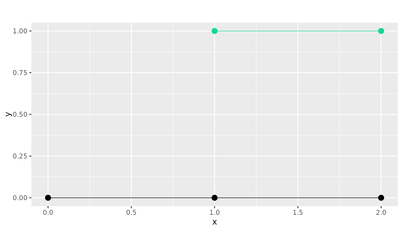
`graph_components$plot()`

Plots all components.

Usage

graph_components$plot(
  edge_colors = NULL,
  vertex_colors = NULL,
  data = NULL,
  ...
)

Arguments

edge_colors: A 3 x nc matrix with RGB values for the edge colors to be used when plotting each graph.
vertex_colors: A 3 x nc matrix with RGB values for the edge colors to be used when plotting each graph.
data: Optional column name of the stored observations to plot. Components without that column are skipped.
...: Additional arguments for plotting the individual graphs.

Returns

A ggplot object.

`graph_components$clone()`

The objects of this class are cloneable with this method.

Usage

graph_components$clone(deep = FALSE)

Arguments

deep: Whether to make a deep clone.

Examples

library(sp)
edge1 <- rbind(c(0, 0), c(1, 0))
edge2 <- rbind(c(1, 0), c(2, 0))
edge3 <- rbind(c(1, 1), c(2, 1))
edges <- list(edge1, edge2, edge3)

suppressWarnings(graphs <- graph_components$new(edges))
#> Starting graph creation...
#> LongLat is set to FALSE
#> Creating edges...
#> Setting edge weights...
#> Computing bounding box...
#> Setting up edges
#> Merging close vertices
#> Total construction time: 0.27 secs
#> Creating and updating vertices...
#> Storing the initial graph...
#> Computing the relative positions of the edges...
#> Extracting components...
#> Number of components: 2
#> Constructing graphs...
#> Processing component 1
#> Starting graph construction...
#> Starting graph creation...
#> LongLat is set to FALSE
#> Creating edges...
#> Setting edge weights...
#> Computing bounding box...
#> Setting up edges
#> Merging close vertices
#> Total construction time: 0.26 secs
#> Creating and updating vertices...
#> Storing the initial graph...
#> Computing the relative positions of the edges...
#> Processing component 2
#> Starting graph construction...
#> Starting graph creation...
#> LongLat is set to FALSE
#> Creating edges...
#> Setting edge weights...
#> Computing bounding box...
#> Setting up edges
#> Merging close vertices
#> Total construction time: 0.26 secs
#> Creating and updating vertices...
#> Storing the initial graph...
#> Computing the relative positions of the edges...
graphs$plot()

Value

Details

Public fields

Methods

Public methods

graph_components$new()

Usage

Arguments

Returns

graph_components$edge_to_component()

Usage

Arguments

Returns

graph_components$get_largest()

Usage

Returns

graph_components$as_metric_graph()

Usage

Returns

graph_components$which_component()

Usage

Arguments

Returns

graph_components$add_observations()

Usage

Arguments

Returns

graph_components$clear_observations()

Usage

Returns

graph_components$get_data()

Usage

Arguments

Returns

graph_components$get_groups()

Usage

Returns

graph_components$get_PtE()

Usage

Returns

graph_components$coordinates()

Usage

Arguments

Returns

graph_components$build_mesh()

Usage

Arguments

Returns

graph_components$compute_fem()

Usage

Arguments

Returns

graph_components$compute_geodist()

Usage

Arguments

Returns

graph_components$compute_resdist()

Usage

Arguments

Returns

graph_components$compute_laplacian()

Usage

Arguments

Returns

graph_components$plot_function()

Usage

Arguments

Returns

graph_components$plot()

Usage

Arguments

Returns

graph_components$clone()

Usage

Arguments

Examples

`graph_components$new()`

`graph_components$edge_to_component()`

`graph_components$get_largest()`

`graph_components$as_metric_graph()`

`graph_components$which_component()`

`graph_components$add_observations()`

`graph_components$clear_observations()`

`graph_components$get_data()`

`graph_components$get_groups()`

`graph_components$get_PtE()`

`graph_components$coordinates()`

`graph_components$build_mesh()`

`graph_components$compute_fem()`

`graph_components$compute_geodist()`

`graph_components$compute_resdist()`

`graph_components$compute_laplacian()`

`graph_components$plot_function()`

`graph_components$plot()`

`graph_components$clone()`