Working with disconnected metric graphs

Introduction

A metric graph need not be connected: real-world networks (street segments, isolated stretches of river, fragmented sensor coverage, etc.) often consist of several disjoint components. The metric_graph class supports this case directly — pass check_connected = FALSE to skip the connectedness warning at construction time, and then use the same methods (add_observations, compute_geodist, compute_resdist, spde_precision, graph_lme, sample_spde, …) as on a connected graph. Distance methods produce Inf for vertex pairs in different components and SPDE precision matrices come out block-diagonal by construction, so no special bookkeeping is required.

This vignette walks through the disconnected workflow: constructing the graph, inspecting and routing across components, computing distances and SPDE models, and per-component visualisation.

For the basics of constructing and working with a single connected metric graph, see Working with metric graphs.

Note. A previous release shipped a separate graph_components class for this purpose. It is deprecated and now emits a warning at construction; the functionality demonstrated below replaces it.

Constructing a disconnected metric graph

We build a small graph with three disjoint components:

Component A is a small “L”-shape with a curved arc.
Component B is a triangle.
Component C is a single straight edge.

# Component A: L-shape with a curved arc
edgeA1 <- rbind(c(0, 0), c(1, 0))
edgeA2 <- rbind(c(0, 0), c(0, 1))
edgeA3 <- rbind(c(0, 1), c(-1, 1))
theta  <- seq(from = pi, to = 3 * pi / 2, length.out = 20)
edgeA4 <- cbind(sin(theta), 1 + cos(theta))

# Component B: a triangle, translated to the right
edgeB1 <- rbind(c(4, 0), c(5, 0))
edgeB2 <- rbind(c(5, 0), c(4.5, 1))
edgeB3 <- rbind(c(4.5, 1), c(4, 0))

# Component C: a single straight edge, placed below
edgeC1 <- rbind(c(1, -2), c(3, -2))

edges <- list(edgeA1, edgeA2, edgeA3, edgeA4,
              edgeB1, edgeB2, edgeB3,
              edgeC1)

Setting check_connected = FALSE suppresses the “graph is disconnected” message:

graph <- metric_graph$new(edges = edges, check_connected = FALSE)
graph$nE

## [1] 8

graph$nV

## [1] 9

The graph behaves exactly like any other metric_graph. Observations, meshes, and SPDE models all work without further setup; the rest of this vignette focuses on the bits that are specific to the disconnected case.

Inspecting the components

get_components() returns the connected components as a list of metric_graph objects. Components are sorted by total edge length, descending:

comps <- graph$get_components()
length(comps)

## [1] 3

sapply(comps, function(g) g$nE)

## [1] 4 3 1

sapply(comps, function(g) sum(as.numeric(g$edge_lengths)))

## [1] 4.570349 3.236068 2.000000

The largest component is just comps[[1]]:

g_largest <- comps[[1]]
g_largest$nE

## [1] 4

For a connected graph, get_components() simply returns list(self), so the same call works uniformly.

Determining the component of a spatial point

which_component() snaps each spatial point to the nearest network location and returns the component index:

XY <- rbind(c(0.5,  0.0),   # near component A
            c(4.5,  0.5),   # inside the triangle (component B)
            c(2.0, -2.0))   # on the bottom edge (component C)
graph$which_component(XY)

## [1] 1 2 3

This is the same routing rule that add_observations() uses internally for spatial input.

Plotting

plot() accepts a components argument that draws every component in a different colour:

graph$plot(components = TRUE)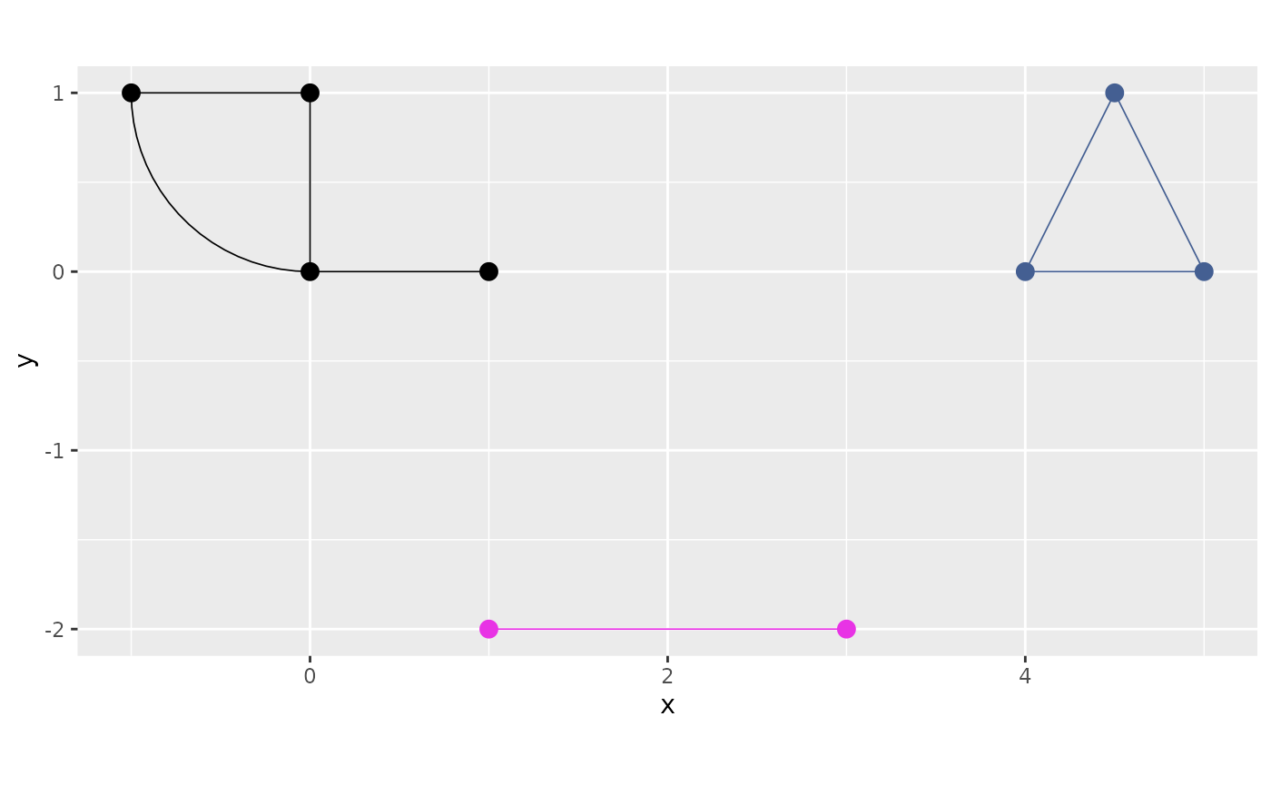

You can also pass an n × 3 matrix of RGB values (one row per component) for explicit colour control:

cols <- rbind(c(0.85, 0.10, 0.10),
              c(0.10, 0.45, 0.85),
              c(0.10, 0.65, 0.20))
graph$plot(components = cols)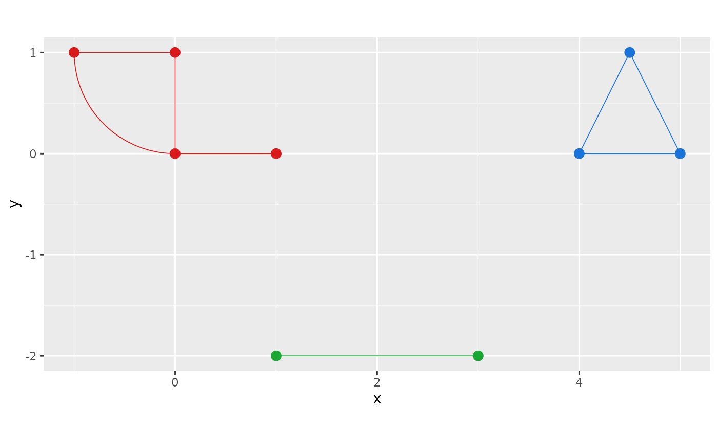

Adding observations

Observations are added with the usual add_observations() method. For data_coords = "spatial" each point is snapped to the nearest edge automatically:

n_obs <- 30
df_spatial <- data.frame(
  coord_x = c(runif(n_obs, -1, 1),
              runif(n_obs,  4,  5),
              runif(n_obs,  1,  3)),
  coord_y = c(runif(n_obs,  0, 1),
              runif(n_obs,  0, 1),
              rep(-2, n_obs)),
  y       = rnorm(3 * n_obs)
)

graph$add_observations(data = df_spatial, data_coords = "spatial",
                       verbose = 0, tolerance = 3)

get_data() returns the observations exactly as for a connected graph. Pair with which_component() if you need a per-component breakdown:

obs <- graph$get_data()
table(graph$which_component(cbind(obs$.coord_x, obs$.coord_y)))

## 
##  1  2  3 
## 30 30 30

For data_coords = "PtE", the usual (edge_number, distance_on_edge) columns are used; edge numbering is global across the whole graph.

Distances on disconnected graphs

compute_geodist() and compute_resdist() are aware that vertices in different components have infinite distance and produce Inf on the cross-component blocks (with finite values within each component):

graph$compute_resdist(full = TRUE)
R <- graph$res_dist[[".complete"]]
# Cross-component pairs are Inf
sum(is.infinite(R)) > 0

## [1] TRUE

# Within-component pairs are finite
all(is.finite(diag(R)))

## [1] TRUE

This means isotropic models such as graph_lme(model = "isoExp") produce exactly zero correlation between components without any special handling.

SPDE models

The SPDE precision matrix spde_precision() builds a per-edge precision matrix and assembles it via vertex indices in graph$E. Because edges in different components touch disjoint vertex sets, the resulting matrix is block-diagonal automatically:

Q <- spde_precision(kappa = 2, tau = 1, alpha = 1, graph = graph)
dim(Q)

## [1] 9 9

# Verify block structure: vertices of component k only connect within k
membership <- igraph::components(
  igraph::make_graph(c(t(graph$E)), directed = FALSE), mode = "weak"
)$membership
cross <- outer(membership, membership, FUN = "!=")
max(abs(as.matrix(Q)[cross]))

## [1] 0

Fitting a Whittle–Matérn model is no different from the connected case:

graph$clear_observations()
df_fit <- data.frame(
  coord_x = c(runif(50, -1, 1), runif(50, 4, 5), runif(50, 1, 3)),
  coord_y = c(runif(50,  0, 1), runif(50, 0, 1), rep(-2, 50)),
  y       = rnorm(150)
)
graph$add_observations(data = df_fit, data_coords = "spatial",
                       verbose = 0, tolerance = 3)

fit <- graph_lme(y ~ 1, graph = graph, model = "WM1")
as.numeric(stats::logLik(fit))

## [1] -211.002

sample_spde() likewise samples a Whittle–Matérn field on a disconnected mesh:

graph$build_mesh(h = 0.1)
graph$compute_fem()
samp <- sample_spde(graph = graph, alpha = 1, kappa = 5, tau = 1,
                    type = "mesh")
graph$plot_function(X = samp, vertex_size = 1)

## Warning: The `X` argument of `plot_function()` is deprecated as of MetricGraph
## 1.3.0.9000.
## ℹ Please use the `newdata` argument instead.
## ℹ The argument `X` is deprecated; please use `newdata` to ensure the correct
##   order when plotting.
## This warning is displayed once per session.
## Call `lifecycle::last_lifecycle_warnings()` to see where this warning was
## generated.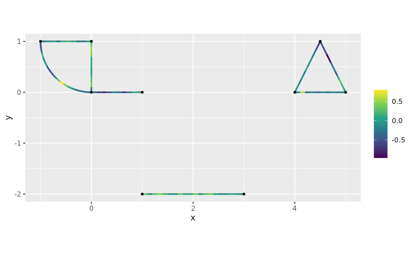

Plotting functions on the components

plot_function() works on disconnected graphs, both for stored data (data = "y") and for an arbitrary newdata indexed by the global .edge_number:

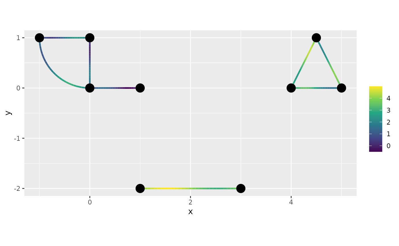
graph$plot_function(data = "y")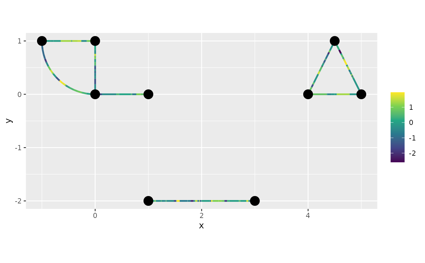

n_per_edge <- 30
newdata <- do.call(rbind, lapply(seq_len(graph$nE), function(e) {
  data.frame(.edge_number      = e,
             .distance_on_edge = seq(0, 1, length.out = n_per_edge))
}))
newdata$f <- with(newdata, sin(2 * pi * .distance_on_edge) + 0.5 * .edge_number)
class(newdata) <- c("metric_graph_data", class(newdata))
graph$plot_function(data = "f", newdata = newdata)

David Bolin, Alexandre B. Simas, and Jonas Wallin

Created: 2026-05-04. Last modified: 2026-05-04.